Signal flow imaging using individual connectome
Contents
1. Introduction
1.1. Scenario
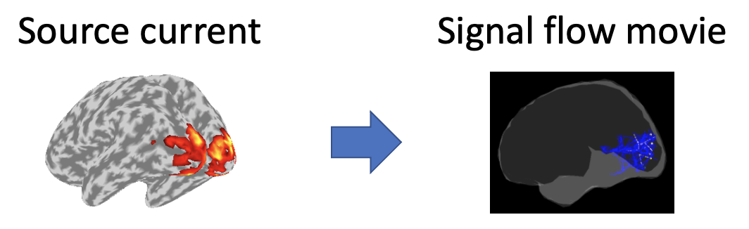
VBMEG can make movies displaying signal flows between brain regions from source currents. Using source currents and a diffusion MRI, this tutorial introduces the procedure to make the signal flow movies. The source currents were estimated from MEG and EEG data during auditory, somatosensory, and visual tasks in M/EEG source imaging. All the procedures will be conducted with scripts.
2. Starting tutorial
2.1. Setting environment
This tutorial was developed using MATLAB 2019a on Linux.
(1) Download and unzip tutorial.zip
(2) Copy and paste all the files to $your_dir
(3) Start MATLAB and change current directory to $your_dir/program
(4) Open make_all.m by typing
>> open make_all
2.2. Adding VBMEG to search path
Thereafter, we will sequentially execute the commands in make_all.m from the top.
We add VBMEG to search path.
>> path_of_VBMEG = '/home/cbi/takeda/analysis/toolbox/vbmeg_20220721';
>> addpath(path_of_VBMEG);
>> vbmeg
Please modify the directories of FSL, jq, MRTrix3, and ANTs written in path_of_VBMEG/vbmegrc for your environment. These softwares will be used in 3.1. dMRI processing.
2.3. Set parameters
We set the parameters for analyzing the dMRI and modeling connectome dynamics, and set the file and directory names.
>> p = set_parameters;
By default, analyzed data and figures will be respectively saved in
- $your_dir/analyzed_data/s006,
- $your_dir/figure.
3. Signal flow imaging
We first calculate anatomical connectivity from the dMRI (3.1 dMRI processing). Then we estimate whole-brain dynamics models using the anatomical connectivity as a constraint (3.2. Modeling connectome dynamics). Finally we create movies displaying signal flows between region of interests (ROIs) (3.3. Creating movie).
3.1. dMRI processing
To obtain anatomical connectivity, which is used as a constraint for modeling connectome dynamics, we analyze the dMRI using FSL and MRtrix3.
Importing dMRI
We convert dMRI DICOM files to a NIfTI (.nii.gz) file.
>> import_dmri(p);
The following files will be saved.
- $your_dir/analyzed_data/s006/dmri/dmri/dmri.nii.gz
- $your_dir/analyzed_data/s006/dmri/dmri/dmri.bval
- $your_dir/analyzed_data/s006/dmri/dmri/dmri.bvec
Preprocessing dMRI
Using mrtrix3_preproc.sh, which runs the recommended preprocessing steps for dMRI and is provided at brainlife, we transform the imported dMRIs into the T1 space and perform motion/eddy-current correction.
>> preproc_dmri(p);
The following files will be saved.
- $your_dir/analyzed_data/s006/dmri/dmri/dwi.nii.gz
- $your_dir/analyzed_data/s006/dmri/dmri/dwi.bvals
- $your_dir/analyzed_data/s006/dmri/dmri/dwi.bvecs
Making brain mask
From the transformed dMRI, we make a mask including brain tissue.
>> make_brain_mask(p);
The following files will be saved.
- $your_dir/analyzed_data/s006/dmri/segment/brain_mask.mif
Making five-tissue-type segmented tissue
Based on the FreeSurfer result, we generate five-tissue-type (5tt) segmented tissue.
>> make_5tt(p);
The following file will be saved.
- $your_dir/analyzed_data/s006/dmri/segment/5tt.mif
Making grey matter-white matter interface
From the 5tt segmented tissue, we generate a mask image for seeding streamlines on the grey matter-white matter interface (gwi).
>> make_gwi(p);
The following file will be saved.
- $your_dir/analyzed_data/s006/dmri/segment/gwi.nii.gz
Estimating response function
We estimate response function for spherical deconvolution.
>> make_response_function(p);
The following file will be saved.
- $your_dir/analyzed_data/s006/dmri/fod/response.mif
Estimating fiber orientation distributions
We estimate fibre orientation distributions (fod) using spherical deconvolution.
>> make_fod(p);
The following file will be saved.
- $your_dir/analyzed_data/s006/dmri/fod/fod.mif
Fiber tracking
Based on the fibre orientation distributions, we execute fiber tracking.
>> fiber_track(p);
The following files will be saved.
- $your_dir/analyzed_data/s006/dmri/fibertrack/fiber1-100.tck
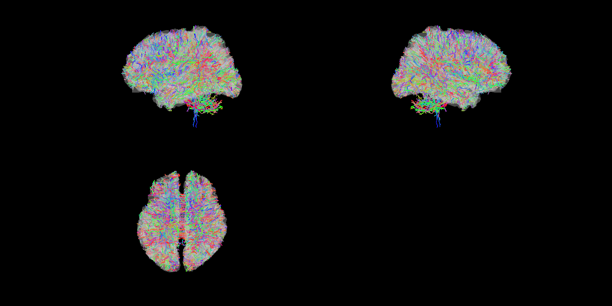
Showing fibers
We show some of the estimated fibers with the brain model.
>> show_fiber(p);
The following figure will be saved.
- $your_dir/figure/show_fiber/s006.png
Mapping fibers to vertices on brain model
We map the estimated fibers to the vertices on the brain model.
>> map_fiber2vertex(p);
The following file will be saved.
- $your_dir/analyzed_data/s006/dmri/fibertrack/corresponding_vertex.mat
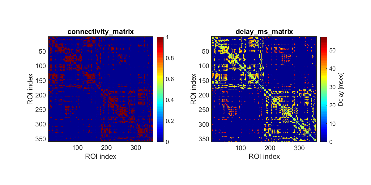
Calculating connectivity
We calculate the connectivity between ROIs, which are defined by HCP-MMP1.0 atlas (Glasser et al., 2016). Furthermore, we calculate the time lags between the ROIs based on the fiber lengths.
>> calculate_connectivity(p);
The following file will be saved.
- $your_dir/analyzed_data/s006/dmri/connectivity/connectivity.mat
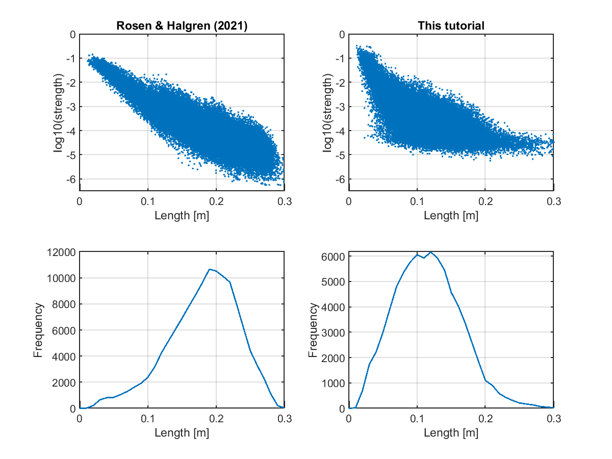
Checking connectivity
We check the estimated connectivity by comparing it with that estimated from a large dataset in Rosen and Halgren (2021).
>> check_connectivity(p);
The following figures will be saved.
- $your_dir/figure/check_connectivity/s006/strength_length.png (Relationship between connectivity strengths and lengths)
- $your_dir/figure/check_connectivity/s006/similarity_of_connectivity_strengths.png
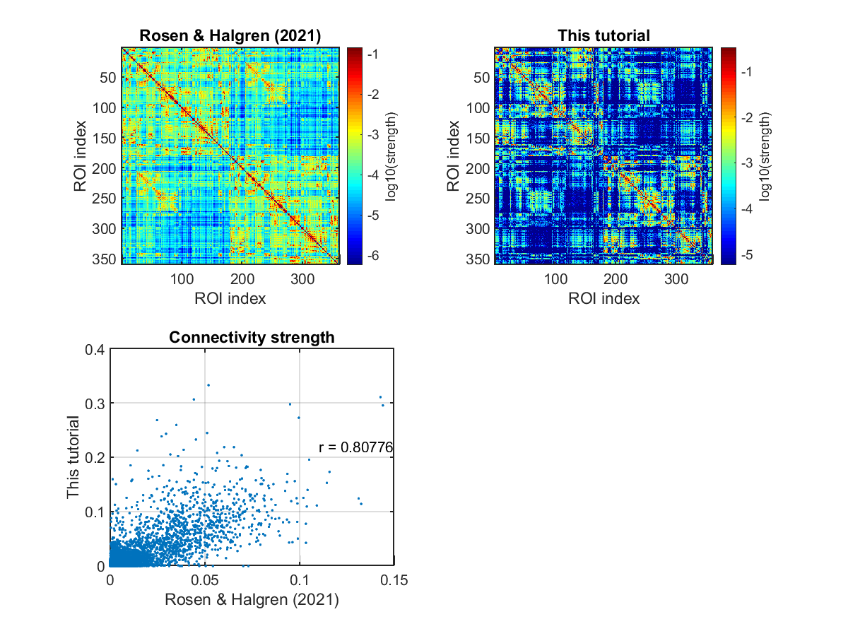
- $your_dir/figure/check_connectivity/s006/binarized_connectivity.png
3.2. Modeling connectome dynamics
From the source currents and the connectivity, we estimate a linear dynamics model (Connectome dynamics estimation).
Calculating ROI-current
We calculate ROI-current by extracting the principal component from the source currents within each ROI.
>> calculate_roi_current(p);
The following files will be saved.
- $your_dir/analyzed_data/s006/dynamics/roi_current/a.mat (Auditory task)
- $your_dir/analyzed_data/s006/dynamics/roi_current/s.mat (Somatosensory task)
- $your_dir/analyzed_data/s006/dynamics/roi_current/v.mat (Visual task)
Estimating dynamics model
From the ROI-current, we estimate a linear dynamics model using the L2-regularized least squares method. In this model, only the anatomically connected pairs of the ROIs have connectivity coefficients (Connectome dynamics estimation).
>> estimate_dynamics_model(p);
The following files will be saved.
- $your_dir/analyzed_data/s006/dynamics/model/a.lcd.mat (Auditory task)
- $your_dir/analyzed_data/s006/dynamics/model/s.lcd.mat (Somatosensory task)
- $your_dir/analyzed_data/s006/dynamics/model/v.lcd.mat (Visual task)
3.2. Creating movie
We create the movies displaying the signal flows between the ROIs (User manual).
Preparing input for creating movie
To create the movies, we need
- The ROI-current,
- The dynamics model,
- The place of the ROIs,
- Time information.
We gather these from separate files.
>> prepare_input_for_movie(p);
The following files will be saved.
- $your_dir/analyzed_data/dynamics/input_for_movie/a.mat (Auditory task)
- $your_dir/analyzed_data/dynamics/input_for_movie/s.mat (Somatosensory task)
- $your_dir/analyzed_data/dynamics/input_for_movie/v.mat (Visual task)
Extracting fiber shapes
To show signal flows along white matter fibers, we extract their shapes between important ROIs from the fiber tracking results.
>> extract_fiber(p);
The following files will be saved.
- $your_dir/analyzed_data/s006/dynamics/fiber/a.mat (Auditory task)
- $your_dir/analyzed_data/s006/dynamics/fiber/s.mat (Somatosensory task)
- $your_dir/analyzed_data/s006/dynamics/fiber/v.mat (Visual task)
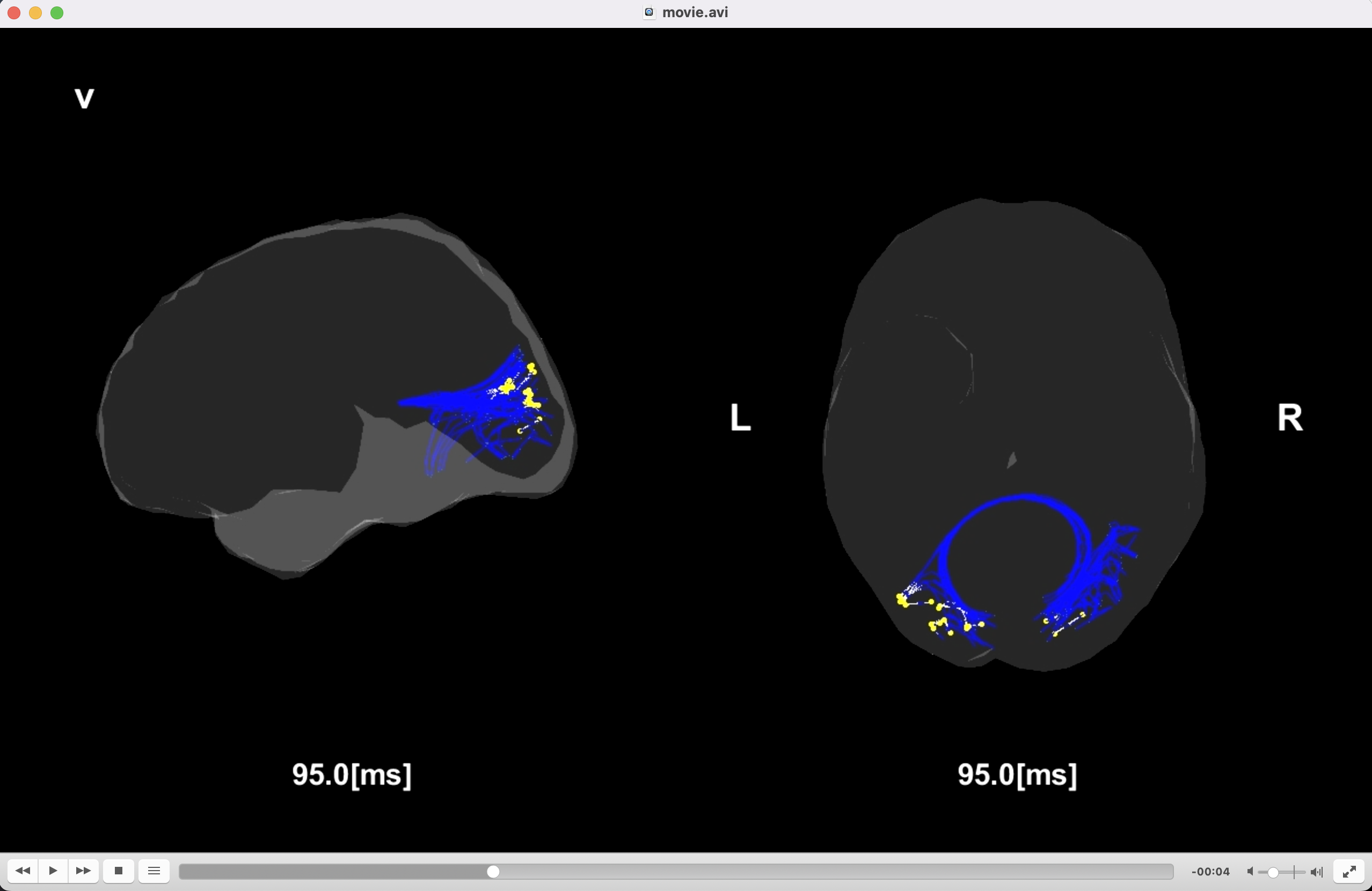
Creating movie
We create the movies displaying the signal flows.
>> create_movie(p);
The following files will be saved.
- $your_dir/analyzed_data/s006/dynamics/movie/a/movie.avi (Auditory task)
- $your_dir/analyzed_data/s006/dynamics/movie/s/movie.avi (Somatosensory task)
- $your_dir/analyzed_data/s006/dynamics/movie/v/movie.avi (Visual task)
Congratulations! You have successfully achieved the goal of this tutorial.