Linear Connectome Dynamics estimation : Two-step method
Linear Connectome Dynamics estimation : Two-step method
The dynamic relationship between current sources at distant position is modeled with a linear dynamics model with connectome constraint and parameters in the model are estimated with the l2-regularized least square method. The dynamics model is described by the following equation.
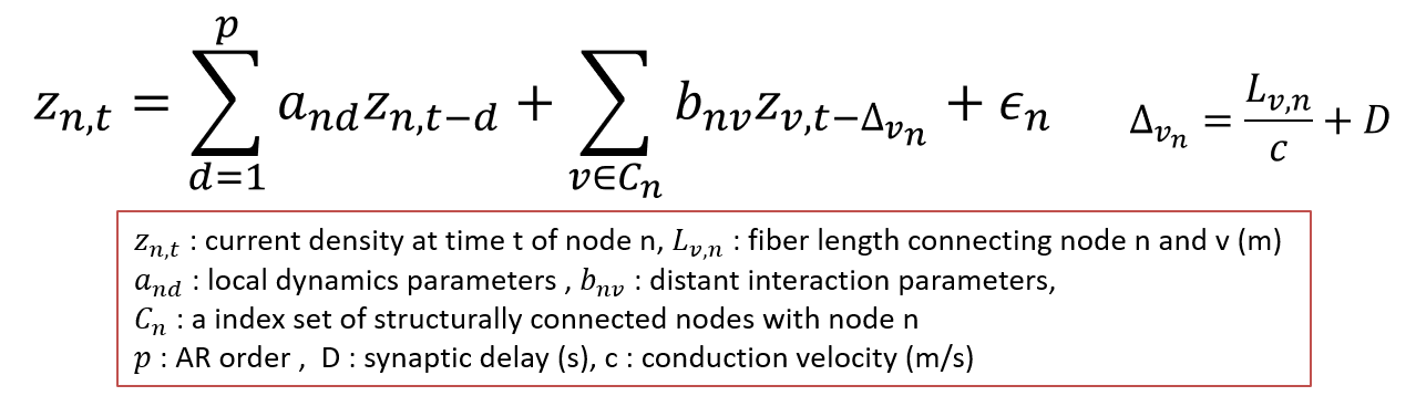
As a default setting, we use p=2, D=20(s), c = 6(m/s) but these values must be explored in the future.
Parameter estimation
[A,B]=lcd_fitl2reg_holocalAR(Z,Delta,2,1e-2*max(sum(Z.^2,2)));
Z is current timeseries (Nv*Nt) (see current source imaging for more details) and Delta is a delay matrix(Nt*Nt)(see dMRI processing for more details). The third and forth argument are local AR order and the regularization parameter common to all the vertices, respectively. A contains local AR coefficients (Nv*p) and B contains effective connectivity (Nv*Nv).
Forward prediction by the estimated model
To see performance of temporal prediction is a good way to validate the estimated parameters. With the following two lines, 50-step ahead predicted current values are obtained using the estimated model. From t=1, Z(:,t) is predicted from Z(:,t-1),...,Z(:,t-maxdelay) using the estimated model. To make prediction for Z(:,1),...,Z(:,maxdelay), zeros are padded at the beginning of Z.
[trs] = lcd_ab2conmar(A, B, Delta, 0); % Form the concatenated MAR matrix (with sparse matrix format)
Zpred = lcd_forward_prediction(trs, Z, 50); % do 50-step prediction repeatedly.
Zpred(:,t) is prediction for Z(:,t). Normalized prediction error for each time step can be calculated as follows.
nerr = sum((Z-Zpred).^2, 1) ./ sum(Z.^2,1); % 1*Nt vector