OSE dataset tutorial
Contents
- Contents
- 1. Introduction
- 2. Start tutorial
- 3. Brain modeling
- 4. SQUID-MEG preprocessing
- 5. EEG preprocessing
- 6. OPM preprocessing
- 7. Solving forward problem
- 8. Solving inverse problem for the auditory and somatosensory task
- 9. Time-frequency analysis for the motor task
1. Introduction
1.1. Scenario
The optically pumped magnetometer (OPM-MEG), SQUID-type magnetoencephalography (SQUID-MEG), and electroencephalography (EEG) are similar measurements but have distinctly different characteristics. We published the OSE dataset, which contains OPM-MEG, SQUID-MEG, and EEG data recorded from the same subjects during multiple tasks. Using this dataset, we could compare OPM-MEG data not only with SQUID-MEG data but also with EEG data, improving our understanding of these measurements comprehensively.
This tutorial guides readers in reproducing the results of our paper of the OSE dataset [Link]. It includes the procedure from importing raw data to performing current source reconstruction for each measurement. In the case of motor task, time-frequency analysis will also be performed. All the procedures will be conducted with scripts.
1.2. Experimental procedure
In the experiment, four subjects performed four tasks:
- Auditory,
- Motor,
- Somatosensory,
- Resting-state.
During the tasks, OPM-MEG measurement was made with 15 OPM sensors, each of which recorded a magnetic field along two axes (Y and Z). SQUID-MEG and EEG were simultaneously recorded with a whole-head 400-channel system (210-channel axial and 190-channel planar gradiometers) and a whole-head 63-channel system, respectively. The horizontal and vertical axes of the electrooculograms (EOGs) and the electromyograms (EMG, only in the motor task to detect the trial onset) were also simultaneously recorded.
For detailed descriptions of the experimental procedure, please see the reference manual of the OSE dataset.
2. Start tutorial
2.1. Setting environment
This tutorial was developed using MATLAB 2021b with Signal Processing Toolbox on Linux.
(1) Download and unzip the OSE dataset from [https://vbmeg.atr.jp/nictitaku209/]
Please download the raw data of all subjects (all.zip), not preprocessed one.
(2) Download and unzip tutorial scripts scripts.zip
(3) Download the latest VBMEG toolbox from here
Please download and install the requirements, including FreeSurfer version 6.0.1 and SPM version 8.
(4) Copy and paste all the files to $your_dir
(4) Start MATLAB and change the current directory to $your_dir/scripts
(5) Open make_all.m by typing
>> open make_all
2.2. Adding toolbox and dataset to the search path
Thereafter, we will sequentially explain the commands in make_all.m from the top.
We recommend executing scripts section by section by clicking "Run Section" button.
In the first section, we add the toolboxes to Matlab's search path.
Please modify each "path_of_VBMEG" and "path_of_SPM8" for your environment.
We also set the directory of the dataset and analysis results.
Please specify the directory of OSEdataset to "dir_dataset" and "dir_result" where you want to save the results.
We note that resulted figures will be saved in $dir_result/figure.
2.3. Setting parameters for EEG/SQUID/OPM analysis
In this section, we set the basic parameters for analysis.
First, we set the subject and task.
In this tutorial, subject "006" and task "Somatosensory" are selected.
If you want to change the subject or task, modify "ss" and "tt" for the corresponding index.
“ss" being 1,2,3,4,5 corresponds to a subject being 002,005,006,093,095, respectively.
“tt" being 1,2,3,4 corresponds to a task being Auditory,Motor,Somatosensory,Rest, respectively.
We note that the pipeline in this tutorial is not for Rest task.
If you analyze Rest, please make a new pipeline for it.
Then, the number of trials is specified.
It is used when we select the same number of trials across all tasks and measurements.
Here, we set 150 trials.
Parameters for the following analysis are pre-defined in "set_parameters.m" function.
If you modify the analysis parameter, please check inside the function.
Returned parameters are struct.
p_eeg = set_parameters(dir_dataset, dir_result, 'eeg', sub, task, num_run_eeg);
p_squid = set_parameters(dir_dataset, dir_result, 'squid', sub, task, num_run_squid);
p_opm = set_parameters(dir_dataset, dir_result, 'opm', sub, task, num_run_opm);
Finally, we add the information about bad channels for OPM and bad ICs for SQUID to the parameters.
These were manually selected.
3. Brain modeling
We make a brain model using T1-weighted MRI data.
Resulted brain model will be used across measurements and tasks.
Therefore, this process should be executed only once for each subject.
When this process is completed, you will see a figure of the brain model superimposed on the MRI image in the directory:
- $dir_result/figure/check_brain_model
Please confirm that the vertices of the brain model represented by the yellow dots are positioned between the grey and white matter.

4. SQUID-MEG preprocessing
In this section, we perform the preprocessing for SQUID-MEG data.
4.1 Importing EEG and SQUID data
First, we import SQUID-MEG data into VBMEG format.
In addition to SQUID, we also import EEG because EOGs are saved in the EEG file.
4.2 Preparation for SQUID data
In this section, we perform some preparation for signal processing.
First, we import EOG data from EEG.
In the case of Motor task, trigger onsets will be detected from EMG data.
Note that the trigger onset is defined as the rise point of EMG measured on the right extensor digitorum muscle.
Then, the trigger signals are rectified with a certain length.
In the case of Auditory task, trigger onsets will be shifted by 20 msec due to delay at ear tubes for sound propagation.
The rectified signal is added as an extra channel named "trigger_modified."
4.3 SQUID preprocessing
We start the SQUID-MEG preprocessing.
In this tutorial, we perform tPCA, prefiltering, ICA, and filtering sequentially.
These processes are performed on the continuous data before it is segmented into trials.
Each preprocess function named "apply_XXX" has a consistent input/output format such as
output_dirname = apply_XXX(p, input_dirname, output_dirname, additional_parameters)
Here, "p" is the parameter struct and "additional_parameters" depends on the preprocessing.
"input_dirname" and "output_dirname" are the name of input and output directory.
By default, they refer to the following directories, respectively.
- $dir_result/$sub/squid-meg/$input_dirname
- $dir_result/$sub/squid-meg/$output_dirname
That is, the preprocessing result of data in the input directory will be saved in the output directory.
Here, we set the name of preprocessing for each directory.
By changing the order of functions, we can easily build our own preprocessing.
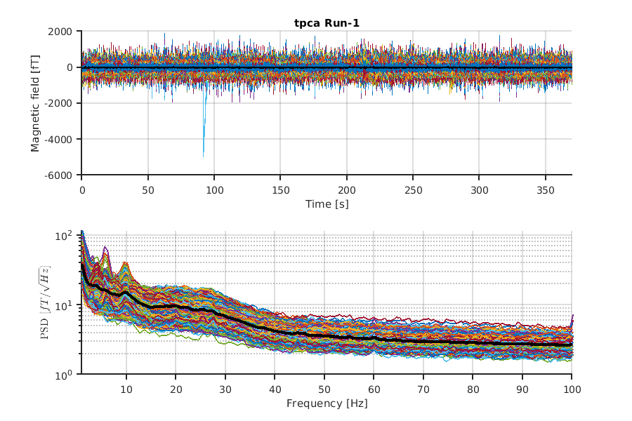
Finally, we visualize the results of preprocessing.
The below function visualizes the result of each step:
show_processed_data(p, dirname, 'NO_REF');
where "dirname" is name of the preprocess and 'NO_REF' indicates "do not show the reference channels."
The figures will be saved in
- $dir_result/figure/show_processed_data
This is an example of tPCA.
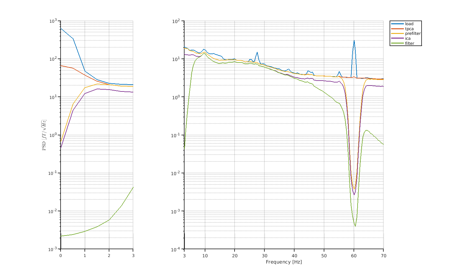
We also compare PSDs of each preprocess.
compare_processed_psd(p_squid, PREP_squid, 'NO_REF');
Here, "PREP_squid" contains all dirnames of preprocessing.
The figures will be saved in
- $dir_result/figure/compare_processed_psd
4.4 SQUID trial-level processing
So far, we have performed signal processing on continuous data.
Here, we first conduct trial segmentation and then perform trial-level processing.
Trial segmentation will be performed on data that have been processed at the last step in section 4.3.
So, we specify the exit point of the pipeline as follows:
pipe_exit = PREP_squid{end};
In this section, processed data will be saved in the bellow directory:
- $dir_result/$sub/squid-meg/trial
Files will be saved by adding the specific prefix.
This means that the file ‘smbr_Somatosensory.info.mat’ is the result of the processes r (rejecting bad channels and trials), b (baseline correction),m (merging run files), and s (selecting trials) executed in sequence.
Hereafter, we explain the processes step by step.
First, we initialize the prefix.
prefix_squid = []; % init prefix
Then, trial segmentation is performed.
make_trial(p_squid, pipe_exit);
In the function, we segment continuous data into trials using the trigger signal.
The results will be saved in
- $dir_result/006/squid-meg/trial/Somatosensory.info.mat
Also, detailed information for trial segmentation will be saved in "pipe_exit" directory.
So, in this case, it is saved in
- $dir_result/006/squid-meg/filter/Somatosensory
Next, we reject bad channels and trials based on data statistics.
prefix_squid = reject_chtr(p_squid, prefix_squid); % prefix:r
For each channel and trial, we make the average of the data during a baseline period to 0.
prefix_squid = correct_baseline(p_squid, prefix_squid); % prefix:b
To handle all the trials collectively, we combine the information of all the trials into a single file (*.info.mat).
prefix_squid = merge_run(p_squid, prefix_squid); % prefix:m
Finally, we select 150 trials randomly to compare measurements with the same number of trials.
prefix_squid = select_trials(p_squid, prefix_squid, num_trial); % prefix:s
After finishing all the above preprocess, we find the time of interest for each task.
"find_temporal_peak.m" will detect the local peaks automatically within the specified time window (p.time_of_interest_sec).
By default, it detects up to three peaks within the window.
However, the user has to decide which of them is the interested response (N20m for Somatosensory, and P50m and N100m for Auditory).
file_peak_squid = find_temporal_peak(p_squid, prefix_squid); % Detected peak of SQUID is used in EEG
In the case of SQUID, detected peaks will be shared with EEG (SQUID and EEG were simultaneously recorded).
Let's check the trial-averaged signals!
show_trial_average(p_squid, prefix_squid);
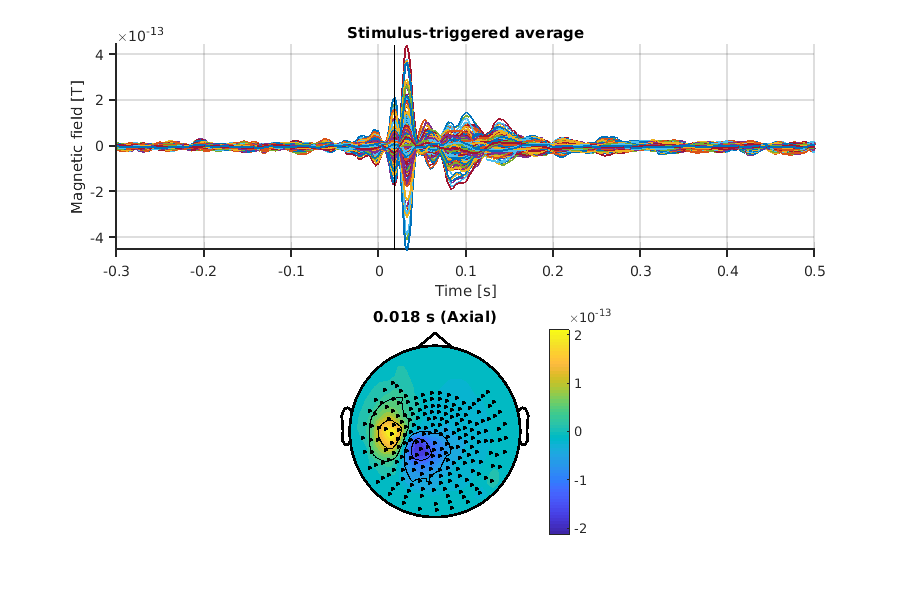
We can see a clear influx/outflux pattern on the left parietal region, a well-known N20m response for SQUID.
5. EEG preprocessing
5.1 Preparation for EEG data
We perform some preparation for EEG data.
For some data, the EOG and trigger signals are saved in the SQUID file, so import them.
Then, the trigger signals are rectified in the same way as the SQUID section.
5.2 EEG preprocessing
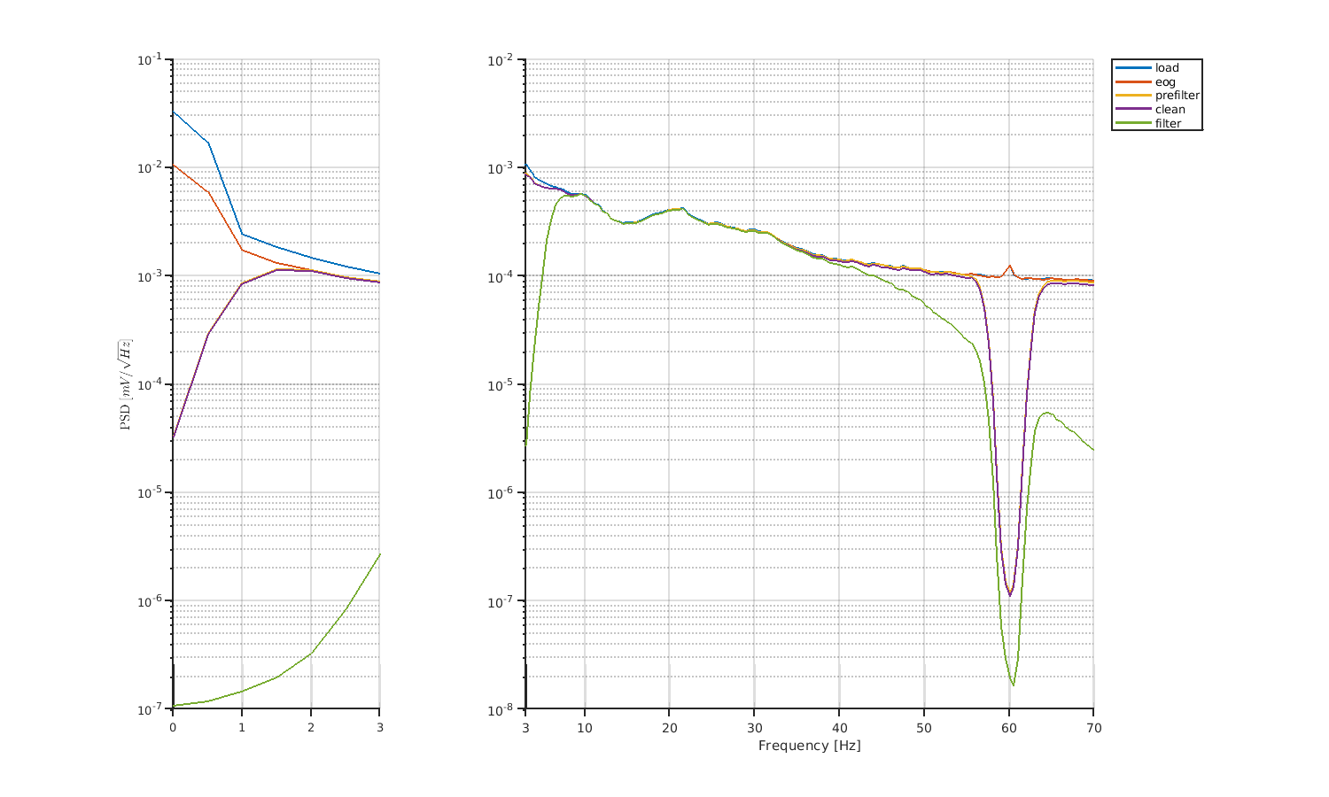
In this tutorial, we perform regressing EOGs, prefiltering, clean channel, and filtering sequentially.
As described in the SQUID section, we can easily modify the pipeline.
You can try other preprocessing methods, such as ICA, if you want.
We note that “apply_XXX_eeg” is a function for EEG, and “apply_XXX_meg” is a function for SQUID or OPM.
Let's check the results of preprocessing by comparing PSDs.
5.3 EEG trial-level processing
The steps are almost the same as for the SQUID section.
One difference is that EEG takes a process for common average reference.
prefix_eeg = common_average_eeg(p_eeg, prefix_eeg); % prefix:c
And it imports the peaks detected by SQUID instead of detecting them using EEG.
find_temporal_peak(p_eeg, prefix_eeg, file_peak_squid);
Let's check the trial-averaged signals.
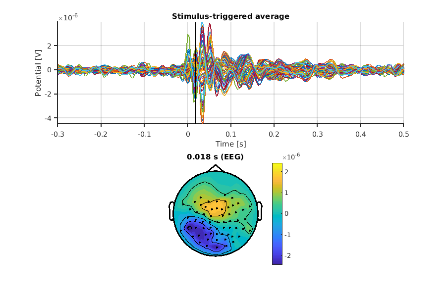
In the case of EEG, we can also observe the peak in the parietal region.
6. OPM preprocessing
6.1 Preparation for OPM data
We start the preparation for OPM data.
Because the OPM-MEG data in the OSE dataset are already in the VBMEG format, we just copy them into the directory of analyzed data.
import_opm(p_opm) {br}
Next, we import EOG data from "eeg.mat" file. {br}
import_eog_opm(p_opm, p_opm.dirname.load) {br}
Then, the trigger signals are rectified with a certain length.
In the case of the auditory task for OPM, trigger onsets will be shifted by 60 msec.
This is because the sound reached the ears 60 msec after the trigger onsets due to a 40-msec delay at a soundboard and a 20-msec delay at ear tubes for sound propagation.
Finally, we import the information of bad channels, which were manually selected.
import_bad_ch(p_opm, p_opm.dirname.load);
6.2 OPM preprocessing
In this tutorial, we perform detrending, regressing EOGs, prefiltering, SSP with VSH2, and filtering sequentially.
As described in the SQUID section, we can easily modify the pipeline.
In the detrending process, we remove large and slow trends from the OPM data using spline interpolation to prevent divergence in the subsequent prefiltering process.
When we apply SSP, output_dirname is stored in "PREP_opm_lf" in addition to "PREP_opm."
This is because SSP requires updating the lead field.
[ PREP_opm{end+1}, PREP_opm_lf{end+1} ] = deal(apply_ssp_meg(p_opm, PREP_opm{end}, p_opm.dirname.ssp, p_opm.ssp));
In our paper, we reported the comparison of SSP basis.
You can try that by modifying the parameter in "p_opm.ssp."
By default, it was set as follows:
p_opm.ssp.ssp_basis = 'VSH'; % Vector Spherical Harmonics
p_opm.ssp.lmax = 2; % Order of VSH
For more information, please check the comment in "apply_ssp_meg.m."
Note that if you want to use "EMPTY" basis, you need to preprocess empty data before that.
Let's check the results of preprocessing by comparing PSDs.
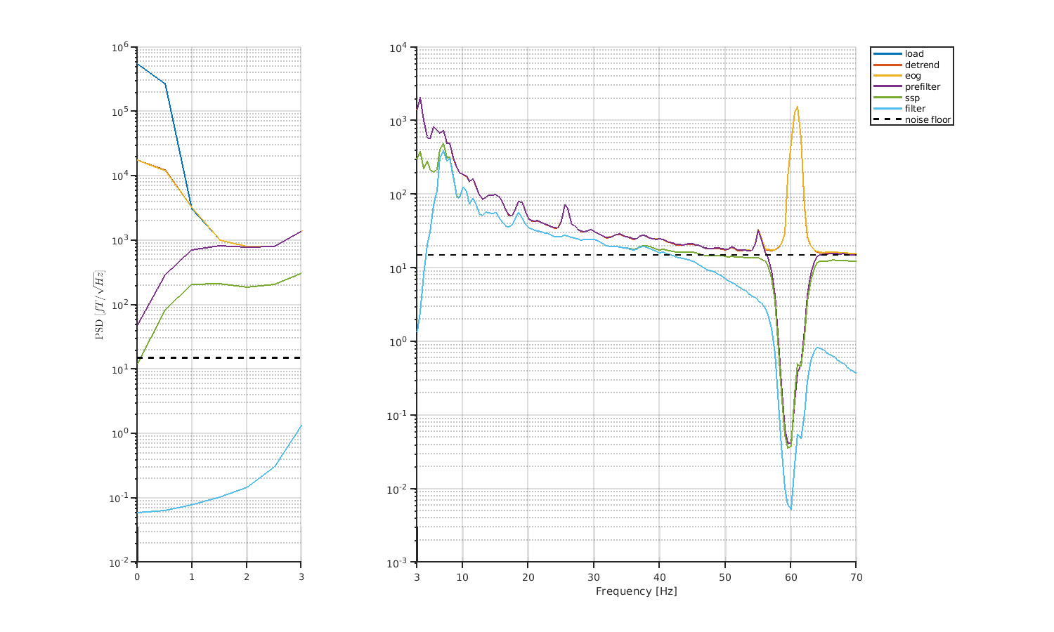
6.3 OPM trial-level processing
The steps are the same as for the SQUID section.
Let's check the trial-averaged signals.
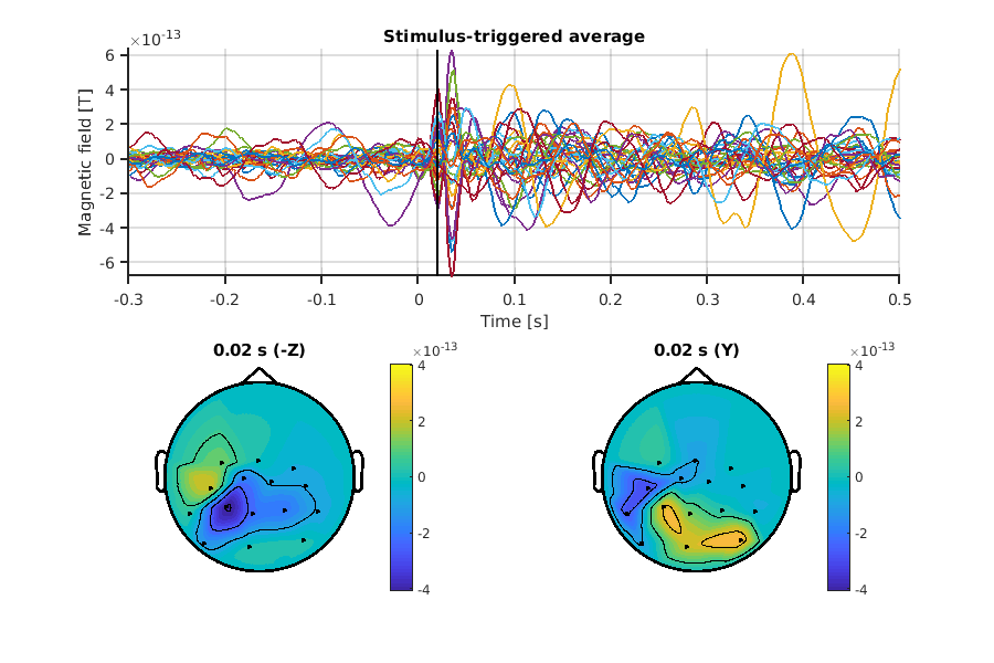
Here, we separately visualize the (-)Z and Y axes.
The derived spatial pattern of Z axis is consistent with SQUID.
7. Solving forward problem
In this section, we will compute a lead field matrix for each measurement using the brain model and sensor positions saved in preprocessed files.
The reason why the lead field is computed task-by-task is to reflect the channel rejection.
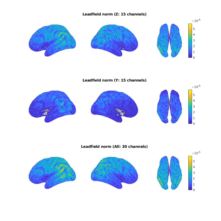
After the computation, we obtain the figures of sensor position (called pick in VBMEG) and lead field norm.
Here, we show the figures of OPM.
In the figure of sensor position, all channels, including inactive channels, were visualized with the direction.
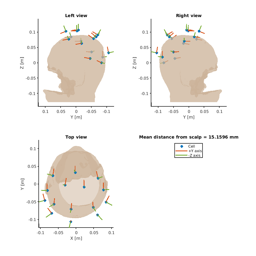
The value of the lead field norm is proportional to the amount of observable signal.
Finally, we update the lead field matrix.
Here, we apply the same projection performed by each SSP to the lead field in the same order.
update_leadfield(p_opm, prefix_opm, PREP_opm_lf{ll}, 'average');
8. Solving inverse problem for the auditory and somatosensory task
In this section, we estimate source currents from MEG/EEG data by dipole-fitting.
In "estimate_source_current_dipole" function, we perform estimation for all time of interest, and both single and double dipole fittings.
Therefore, please use an appropriate result for the task.
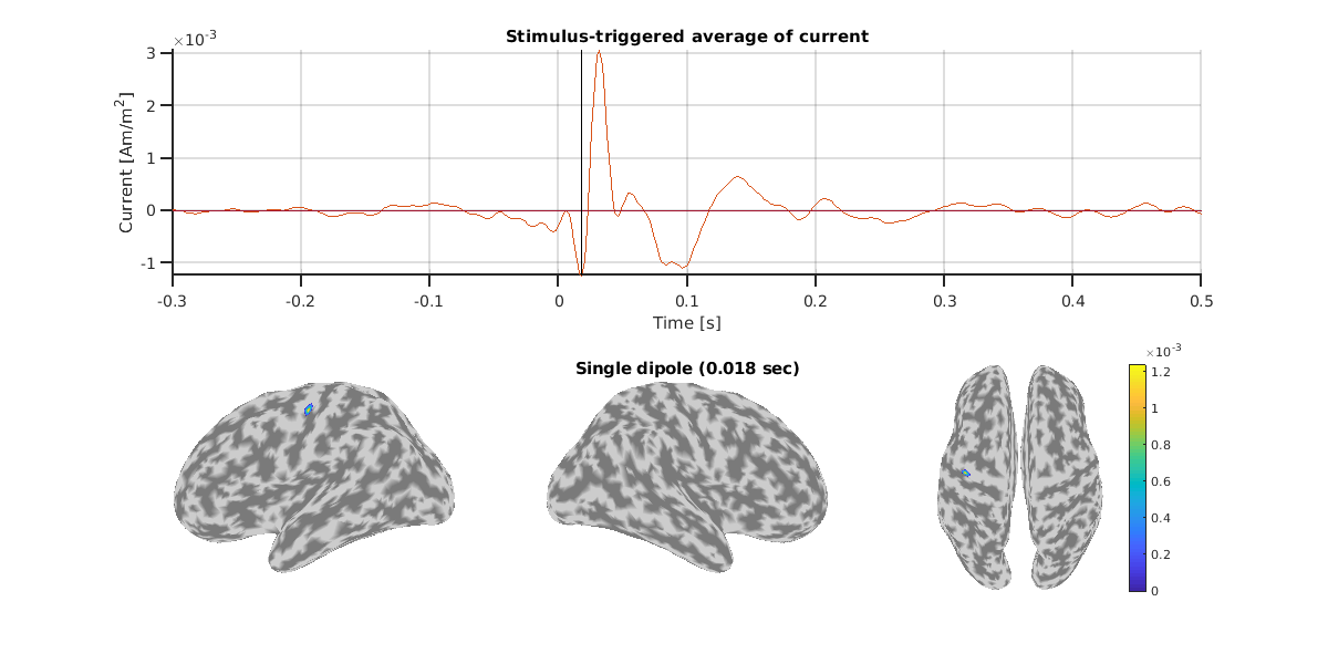
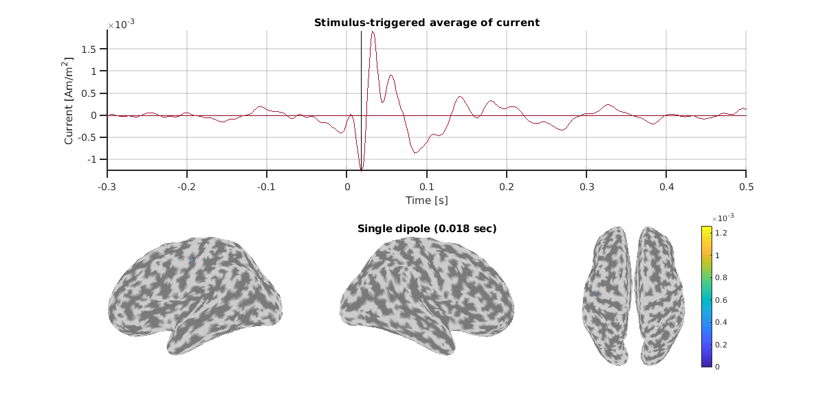
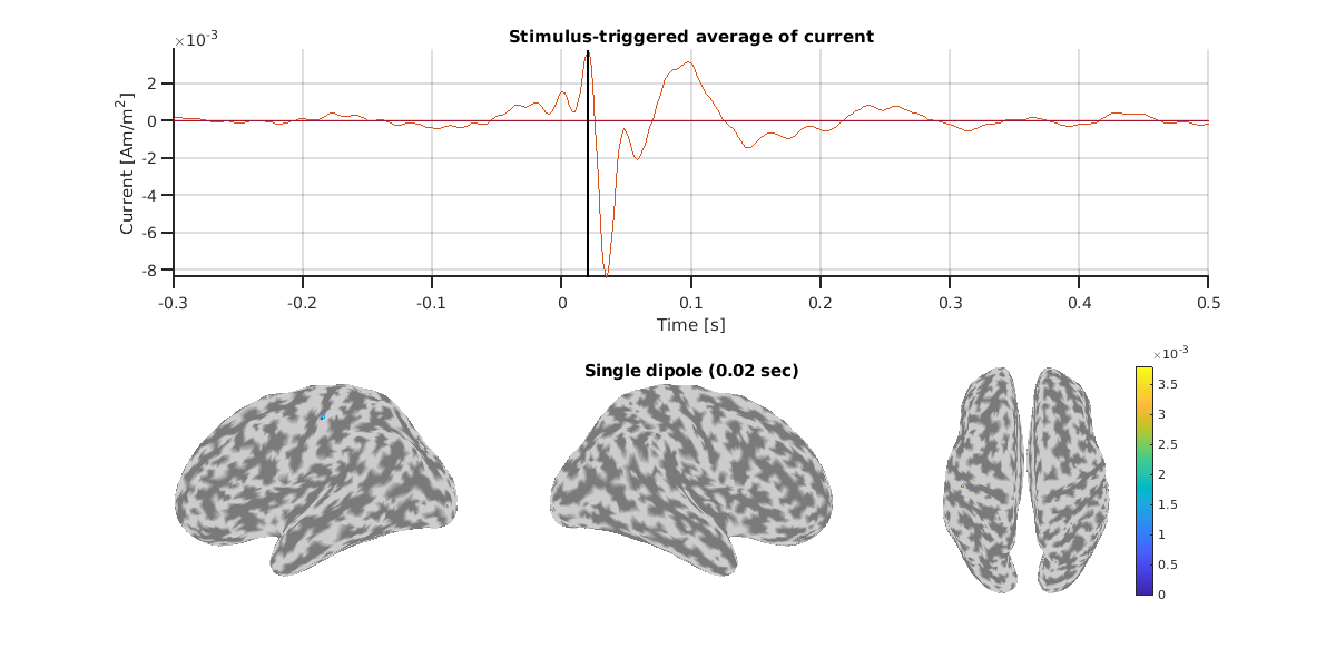
Here, let's check the estimated single dipole of N20m.
For this subject, we can confirm consistent dipoles around the left central gyrus across measurements.
Result of SQUID.
Result of EEG.
Result of OPM.
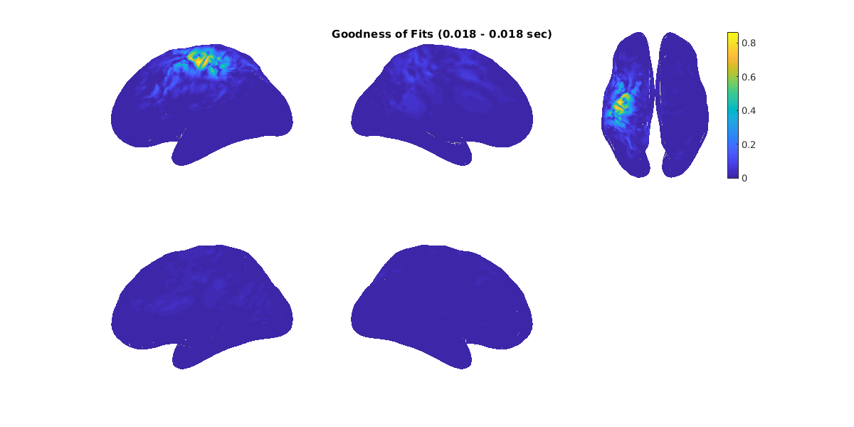
The goodness of fit of single-dipole is also visualized.
If you want to perform other source localization methods, please check "estimate_source_current_VBMEG.m" or "estimate_source_current_SOLCO.m."
In the former, hierarchical Bayesian estimation implemented in VBMEG can be tried.
In the latter, various source localization methods (e.g., LCMV beamformer) implemented by us can be tried.
9. Time-frequency analysis for the motor task
In this section, we perform a time-frequency analysis for the motor task.
Before conducting this, we need to perform all the preprocessing for the motor task.
Here, we use the motor task of subject 002 as an example.
Note that much RAM and write space will be consumed here.
For the first, we make "tfr.mat" files using preprocessed data.
These are time-frequency decomposition of the sensor signal, which adds an axis of frequency to the original data.
In this tutorial, we use Wavelet decomposition.
make_tfr(p_squid, PREP_squid{end}, prefix_squid);
make_tfr(p_opm, PREP_opm{end}, prefix_opm);
make_tfr(p_eeg, PREP_eeg{end}, prefix_eeg);
After computing TFR files, we visualize them.
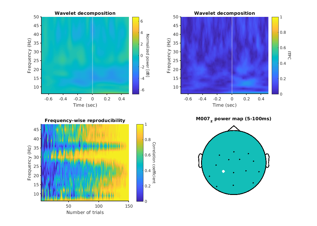
As an example, we show the left parietal channel of the OPM.
Left top panel shows the result of Wavelet decomposition.
The color bar appears weak, as it is shared across all channels, but ERD can be observed in the alpha band.
Right top panel indicates the intertrial phase coherence, left bottom panel is frequency-wise reproducibility, and right bottom panel is the position of the channel.
To perform the DICS beamformer, we set the time and frequency of interest.
The time of interest (toi) is set to 0.1-0.4 sec for all subjects.
toi_sec = [ 0.1 0.4 ];
The frequency of interest (foi) is specified for each subject because of subject-dependency and artifacts.
We set 15-18 Hz for subject 002.
foi_hz = [ 15 18 ];
Finally, we perform the DICS beamformer.
estimate_source_current_freq(p_squid, prefix_squid, toi_sec, foi_hz);
estimate_source_current_freq(p_opm, prefix_opm, toi_sec, foi_hz);
estimate_source_current_freq(p_eeg, prefix_eeg, toi_sec, foi_hz);
By using "show_source_current_freq.m," we can check the estimated currents.
Here we see the pseudo-F-ratio map of ERS and ERD for OPM.
If you want to change the visualization, please check the options for "show_source_current_freq.m."

Congratulations! You have successfully completed all the steps in this tutorial.
Enjoy further analysis with other tasks and other subjects by making your own analysis!