OPM processing
Contents
1. Introduction
1.1. Scenario
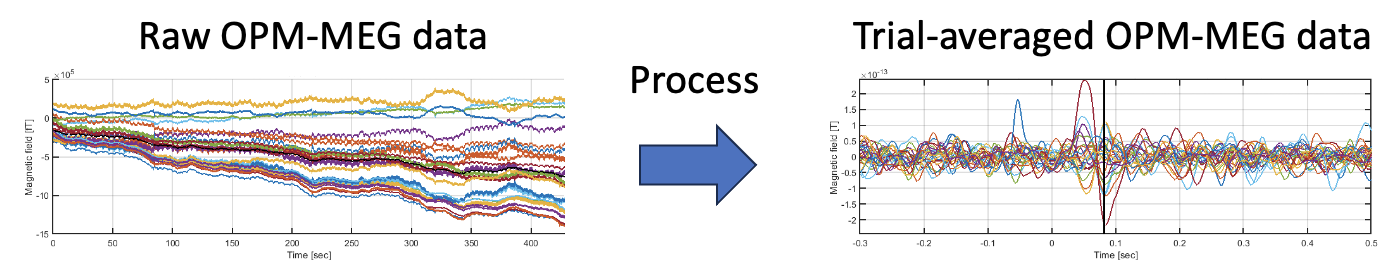
An optically pumped magnetometer (OPM) is a new type of magnetoencephalography (MEG) device, which enables a wearable MEG measurement system. Using OPM-MEG data in the OPM-MEG, SQUID-MEG, and EEG (OSE) dataset, this tutorial guides through the procedures from importing raw OPM-MEG data to showing trial-averaged OPM-MEG data. All the procedures will be conducted with scripts.
1.2. Experimental procedure
In the experiment, four subjects performed four tasks:
- Auditory,
- Motor,
- Somatosensory,
- Resting-state.
During the tasks, the OPM-MEGs were recorded with 15 OPM sensors, each of which recorded a magnetic field along two axes (Y and Z). Electrooculograms (EOGs) were also recorded simultaneously.
For detailed descriptions of the experimental procedure, please see the reference manual of the OSE dataset.
This tutorial analyzes the OPM-MEG data during the auditory, motor, and somatosensory tasks.
2. Start tutorial
2.1. Set environment
This tutorial was developed using MATLAB 2019a with Signal Processing Toolbox on Linux.
(1) Download the latest VBMEG toolbox from here
(2) Download and unzip tutorial.zip
(3) Copy and paste all the files to $your_dir
(4) Start MATLAB and change the current directory to $your_dir/program
(5) Open make_all.m by typing
>> open make_all
2.2. Add necessary toolboxes to the search path
Thereafter, we will sequentially execute the commands in make_all.m from the top.
We add the VBMEG toolbox to the search path.
>> path_of_VBMEG = '/home/cbi/takeda/analysis/toolbox/vbmeg_20231120';
>> addpath(path_of_VBMEG);
>> vbmeg
Please modify path_of_VBMEG for your environment.
We also add all the directories in the current directory to the search path.
>> addpath(genpath(cd))
2.3. Set parameters
We get the properties of the OPM-MEG dataset, such as subject and task names.
>> d = define_dataset;
Based on the properties, we set the subject, task, and number of runs.
>> ss = 1;% 1, 2, 3, or 4
>> sub = d.sub_list{ss};
>> tt = 1;% 1: Auditory, 2: Motor, or 3: Somatosensory
>> task = d.task_list{tt};
>> num_run = d.num_run_table_opm{sub, task};
Then, we set the parameters and directory names for analyzing the OPM-MEG data.
>> p = set_parameters(sub, task, num_run);
By default, analyzed data and figures will be respectively saved in
- $your_dir/analyzed_data/002,
- $your_dir/analyzed_data/figure.
Finally, we add the information about bad channels to the parameters. The bad channels were manually selected.
>> p = set_bad_ch(p);
3. Process OPM-MEG data
3.1. Import OPM-MEG data
Because the OPM-MEG data in the OSE dataset are already in the VBMEG format, we just copy them into the directory of analyzed data.
>> import_opm(p)
The following files will be saved.
- $your_dir/analyzed_data/002/load/Auditory/run01.meg.mat (OPM-MEG, run 1)
- $your_dir/analyzed_data/002/load/Auditory/run01.eeg.mat (EOG, run 1)
- $your_dir/analyzed_data/002/load/Auditory/run02.meg.mat (OPM-MEG, run 2)
- $your_dir/analyzed_data/002/load/Auditory/run02.eeg.mat (EOG, run 2)
3.2. Import EOG data
Because the EOG was recorded with an electroencephalography (EEG) device, we import the EOG data from the EEG file into the OPM-MEG file.
>> import_eog(p, p.dirname.load)
The EOG data will be added in the imported OPM-MEG file as extra-channel data (bexp_ext).
3.3. Modify trigger signal
We modify the trigger signal so that stimulus onsets can be appropriately detected in making trial data. In the case of the auditory task, trigger onsets will be shifted by 60 msec. This is because the sound reached the ears 60 msec after the trigger onsets due to a 40-msec delay at a soundboard and a 20-msec delay at ear tubes for sound propagation.
>> if strcmp(p.task, 'Auditory')
>> modify_trigger(p, p.dirname.load, 60); % Shift 60 msec
>> else
>> modify_trigger(p, p.dirname.load);
>> end
The modified trigger signal will be also added in the imported OPM-MEG file as the extra-channel data (bexp_ext).
3.4. Import bad-channel information
We import the information of bad channels, which were manually selected.
>> import_bad_ch(p, p.dirname.load);
The bad-channel information will be added to a struct (MEGinfo) in the imported OPM-MEG file.
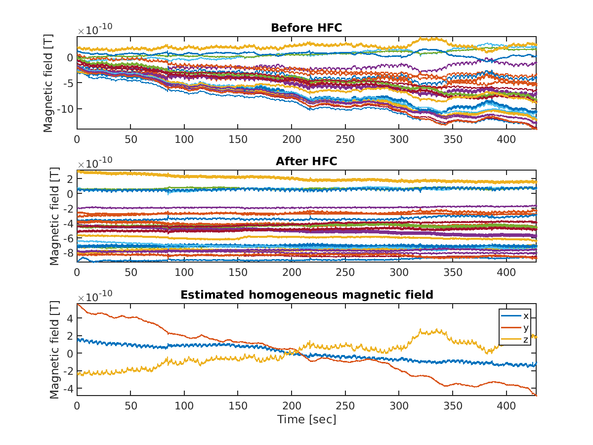
3.5. Homogeneous field correction
To remove environmental noise, we apply homogeneous field correction (HFC) (Tierney et al., 2021 Neuroimage) to the OPM-MEG data.
>> PREP{end+1} = apply_hfc(p, PREP{end}, p.dirname.hfc);
The following files and figures will be saved.
- $your_dir/analyzed_data/002/hfc/Auditory/run01.meg.mat
- $your_dir/analyzed_data/002/hfc/Auditory/run02.meg.mat
- $your_dir/analyzed_data/figure/apply_hfc/Auditory/002_run01_hf.png
- $your_dir/analyzed_data/figure/apply_hfc/Auditory/002_run02_hf.png
For the motor task, we skip HFC because it seems to remove motor-related brain activities as well as noise.
3.6. Detrend OPM-MEG data
To prevent the divergence in the subsequent filtering process, we remove large and slow trends from the OPM-MEG data using spline interpolation.
>> PREP{end+1} = apply_detrending(p, PREP{end}, p.dirname.detrend);
The following files will be saved.
- $your_dir/analyzed_data/002/detrend/Auditory/run01.meg.mat
- $your_dir/analyzed_data/002/detrend/Auditory/run02.meg.mat
3.7. Filter OPM-MEG data
The OPM-MEG data include large noises, such as the line noise (60 Hz at Kansai in Japan). To remove these noises, we apply bandstop and bandpass filters.
>> PREP{end+1} = apply_filtering(p, PREP{end}, p.dirname.filter);
The following files will be saved.
- $your_dir/analyzed_data/002/filter/Auditory/run01.meg.mat
- $your_dir/analyzed_data/002/filter/Auditory/run02.meg.mat
3.8. Show processed OPM-MEG data
We check the time series and power spectral densities (PSDs) of the processed OPM-MEG data at each stage.
>> for pp = 1:length(PREP)
>> show_processed_data(p, PREP{pp});
>> end
Figures will be saved in
- $your_dir/analyzed_data/figure/show_processed_data/Auditory.
Furthermore, we compare the PSDs across the stages.
>> compare_processed_psd(p, PREP);
The following figures will be saved.
- $your_dir/analyzed_data/figure/compare_processed_psd/Auditory/002_run01.png
- $your_dir/analyzed_data/figure/compare_processed_psd/Auditory/002_run02.png

3.9. Make trial data
We segment the continuous OPM-MEG data into trials (epochs). First, we detect stimulus onsets from the trigger signals included in the extra-channel data. Then, we segment the OPM-MEG data into trials by the detected stimulus onsets.
>> make_trial(p, PREP{end});
The following files will be saved.
- $your_dir/analyzed_data/002/trial/Auditory/run01.meg.mat
- $your_dir/analyzed_data/002/trial/Auditory/run02.meg.mat
3.10. Reject bad channels and trials
We reject bad channels and trials based on data statistics.
>> prefix = []; % Initialize prefix
>> prefix = reject_chtr(p, prefix, PREP{end});
The following files will be saved.
- $your_dir/analyzed_data/002/trial/Auditory/r_run01.meg.mat
- $your_dir/analyzed_data/002/trial/Auditory/r_run02.meg.mat
3.11. Regress out EOG component from OPM-MEG data
We regress out EOG components from the OPM-MEG data. For each channel, we construct a linear model to predict the OPM-MEG data from the EOG data and remove the prediction from the OPM-MEG data.
>> prefix = regress_out_eog(p, prefix);
The following files will be saved.
- $your_dir/analyzed_data/002/trial/Auditory/er_run01.meg.mat
- $your_dir/analyzed_data/002/trial/Auditory/er_run02.meg.mat
3.12. Correct baseline
For each channel and trial, we make the average of the OPM-MEG data during a baseline period to 0.
>> prefix = correct_baseline(p, prefix);
The following files will be saved.
- $your_dir/analyzed_data/002/trial/Auditory/ber_run01.meg.mat
- $your_dir/analyzed_data/002/trial/Auditory/ber_run02.meg.mat
3.13. Combine trials across runs
To handle all the trials collectively, we combine the information of all the trials into a single file (*.info.mat).
>> prefix = combine_trial(p, prefix);
The following file will be saved.
- $your_dir/analyzed_data/002/trial/ber_Auditory.info.mat
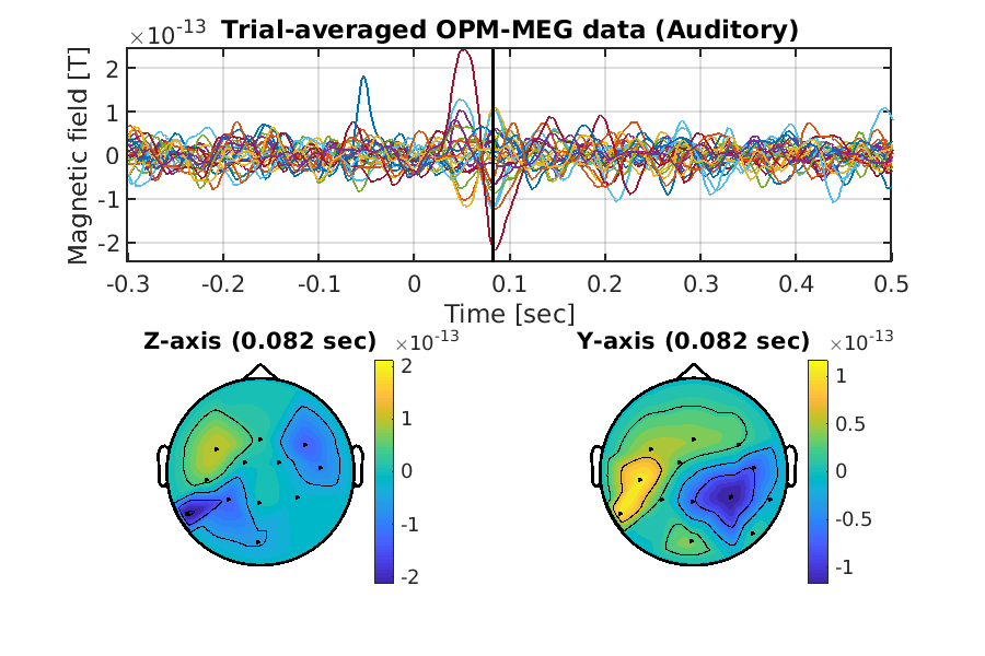
3.14. Show trial-averaged OPM-MEG data
Finally, we show the processed OPM-MEG data averaged across the trials.
>> show_trial_average(p, prefix);
The following figure will be saved.
- $your_dir/analyzed_data/figure/show_trial_average/Auditory/002.png
Congratulations! You have successfully achieved the goal of this tutorial.