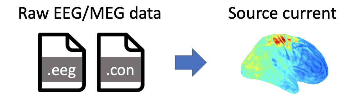
Source imaging from resting-state M/EEG data

Contents
1. Introduction
2. Starting tutorial
3. Modeling brain
4. Source imaging from EEG data
5. Source imaging from MEG data
6. Source imaging from both EEG and MEG data

1. Introduction

1.1. Scenario

Using VBMEG's functions, this tutorial demonstrates the source imaging from resting-state EEG and MEG data by the Linearly Constrained Minimum Variance (LCMV) beamformer (Van Veen et al., 1997). All the procedures will be conducted with scripts.

1.2. Experimental procedure

A subject performed a resting-state task, in which he fixated on a cross for about five minutes.

During the task, EEG and MEG were simultaneously recorded with a whole-head 63-channel system (BrainAmp; Brain Products GmbH, Germany) and a whole-head 400-channel system (210-channel Axial and 190-channel Planar Gradiometers; PQ1400RM; Yokogawa Electric Co., Japan), respectively. The sampling frequency was 1 kHz. Electrooculogram (EOG) signals were also simultaneously recorded and included in the EEG file.

Using three Three Tesla MR scanner (MAGNETOM Prisma, Siemens, Erlangen, Germany), we also conducted an MRI experiment to obtain a T1-weighted image.

2. Starting tutorial

2.1. Setting environment

This tutorial was developed using MATLAB 2019a on Linux.

(1) Download and unzip tutorial.zip
(2) Copy and paste all the files to $your_dir
(3) Start MATLAB and change current directory to $your_dir/program
(4) Open make_all.m by typing

>> open make_all

2.2. Adding paths

Thereafter, we will sequentially execute the commands in make_all.m from the top.

We set directories of necessary toolboxes: VBMEG and SPM8. Please modify these for your environment.

>> path_of_VBMEG = '/home/cbi/takeda/analysis/toolbox/vbmeg_20220721';
>> path_of_SPM8 = '/home/cbi-data20/common/software/external/spm/spm8';

Please modify the directories of FreeSurfer written in path_of_VBMEG/vbmegrc for your environment and execute the following commands to add the toolboxes to search path.

>> addpath(path_of_VBMEG);
>> vbmeg
>> addpath(path_of_SPM8);

2.3. Setting parameters

We set the parameters for analyzing the EEG and MEG data and set the file and directory names.

>> p = set_parameters

By default, processed data and figures will be respectively saved in

$your_dir/analyzed_data,
$your_dir/figure.

3. Modeling brain

First of all, we construct a cortical surface model from the T1 image and define current sources on it.

3.1. Importing T1-weighted image

We import a T1-weighted image by copying the T1 file (.nii) from original_data to analyzed_data.

>> import_T1(p);

The following file will be saved.

$your_dir/analyzed_data/T1/Subject.nii

3.2. Correcting bias in T1-weighted image

Using SPM8, we correct bias in the T1-weighted image (User manual).

>> correct_bias_in_T1(p);

The following file will be saved.

$your_dir/analyzed_data/T1/mSubject.nii

3.3. Segmenting T1-weighted image

Using SPM8, we extract a gray matter image from the T1-weighted image.

>> segment_T1(p);

The following file will be saved.

$your_dir/analyzed_data/T1/c1mSubject.nii (Gray matter)

This file will be used in 4.3 Preparing leadfield matrix.

3.4. Constructing cortical surface model from T1-weighted image

Using FreeSurfer, we construct a polygon model of the cortical surface from the T1-weighted image (User manual).

>> construct_cortical_surface_model(p);

The generated files will be saved in

$your_dir/analyzed_data/FS.

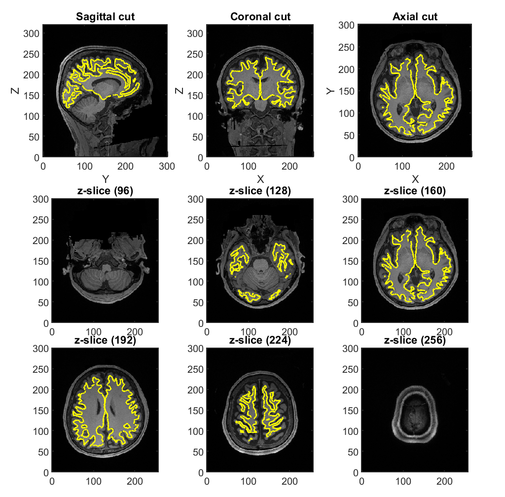
3.5. Constructing brain model from the cortical surface model

From the cortical surface model, we construct a brain model, in which the positions of current sources are defined on the cortical surface (vb_job_brain.m).

>> construct_brain_model(p);

The following files and figure will be saved.

$your_dir/analyzed_data/brain/Subject.brain.mat (Brain model)
$your_dir/analyzed_data/brain/Subject.act.mat (Prior information)
$your_dir/analyzed_data/brain/Subject.area.mat (Area information)
$your_dir/analyzed_data/brain/Subject.png

4. Source imaging from EEG data

In this section, we introduce the procedures to estimate the source current from the resting-state EEG data.

4.1. Importing EEG data

We convert BrainAmp files to MAT files (User manual, vb_job_meg.m).

>> import_eeg(p);

The following file will be saved.

$your_dir/analyzed_data/EEG/imported/run01.eeg.mat

4.2. Filtering EEG data

The recorded EEG data includes drift and line noise (60 Hz at Kansai in Japan). To remove these noises, we apply a low-pass filter, down-sampling, and a high-pass filter.

>> filter_eeg(p);

The following file will be saved.

$your_dir/analyzed_data/EEG/filtered/run01.eeg.mat

4.3. Preparing leadfield matrix

We make a leadfield matrix, a tranformation matrix from the source current to the EEG data. First, we construct a 3-shell (cerebrospinal fluid, skull, and scalp) surface model (User manual, vb_job_head_3shell.m). Then, we make the leadfield matrix based on the 3-shell model (User manual, vb_job_leadfield.m).

>> prepare_leadfield_eeg(p);

The following files will be saved.

$your_dir/analyzed_data/EEG/leadfield/Subject.head.mat (3-shell model)
$your_dir/analyzed_data/EEG/leadfield/Subject.basis.mat (Leadfield matrix)

4.4. Collecting data

We collect the necessary data for the source imaging (e.g. the EEG data and the leadfield matrix). Hereafter, the data will be saved in a simple format rather than the VBMEG's.

>> collect_data_eeg(p);

The following file will be saved.

$your_dir/analyzed_data/EEG/collected/run01.mat

4.5. Removing EOG components

We regress out EOG components from the EEG data. For each channel, we construct a linear model to predict the EEG data from the EOG data and remove the prediction from the EEG data.

>> remove_eog_eeg(p);

The following file will be saved.

$your_dir/analyzed_data/EEG/eog_removed/run01.mat

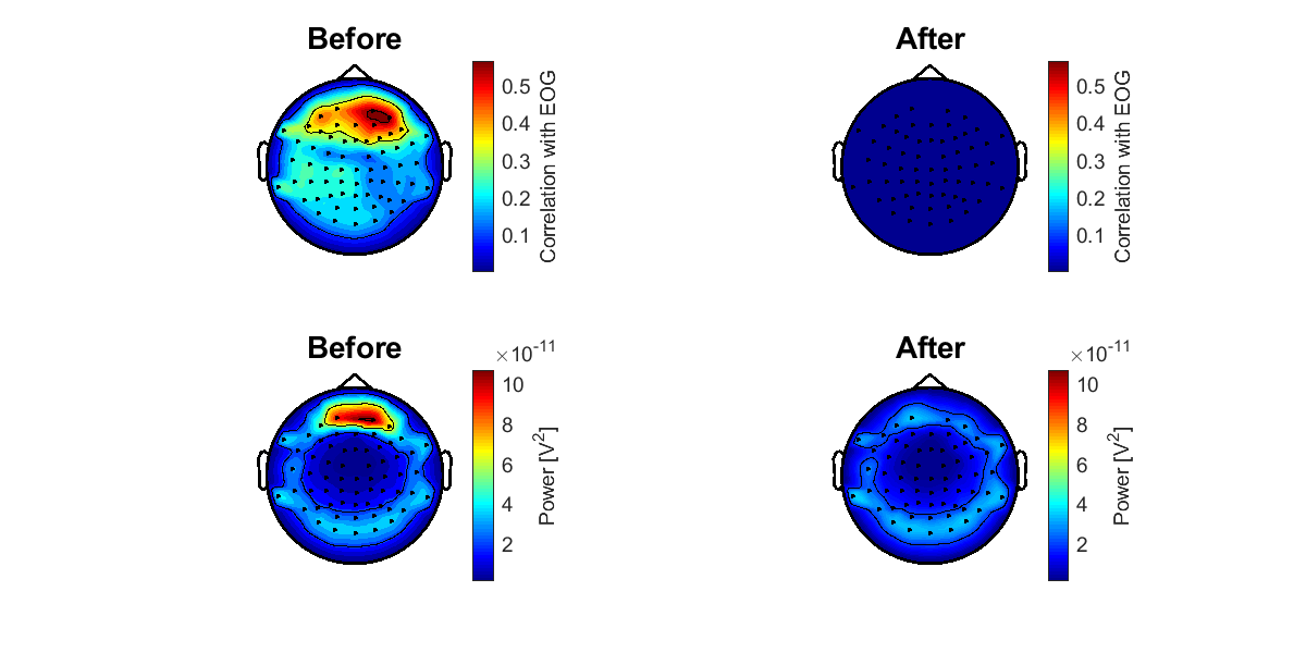
4.6. Checking the result of removing EOG components

To check whether the EOG components were appropriately removed, we calculate the correlation coefficients between the EEG data at each channel and the EOG data. The correlation coefficients are shown on the sensor space (vb_plot_sensor_2d.m).

>> check_eog_removed_eeg(p);

The following figure will be saved.

$your_dir/figure/check_eog_removed_eeg.png

4.7. Removing bad channels

We remove noisy channels.

>> remove_bad_ch_eeg(p);

The following file will be saved.

$your_dir/analyzed_data/EEG/bad_ch_removed/run01.mat

4.8. Estimating source current

We estimate the source current from the preprocessed EEG data. First, we take common average; that is, we make the averages of the EEG data and the leadfield matrix across the channels to 0. Then, we applied the LCMV beamformer.

>> estimate_current_eeg(p);

The following file will be saved.

$your_dir/analyzed_data/EEG/source_current/run01.mat

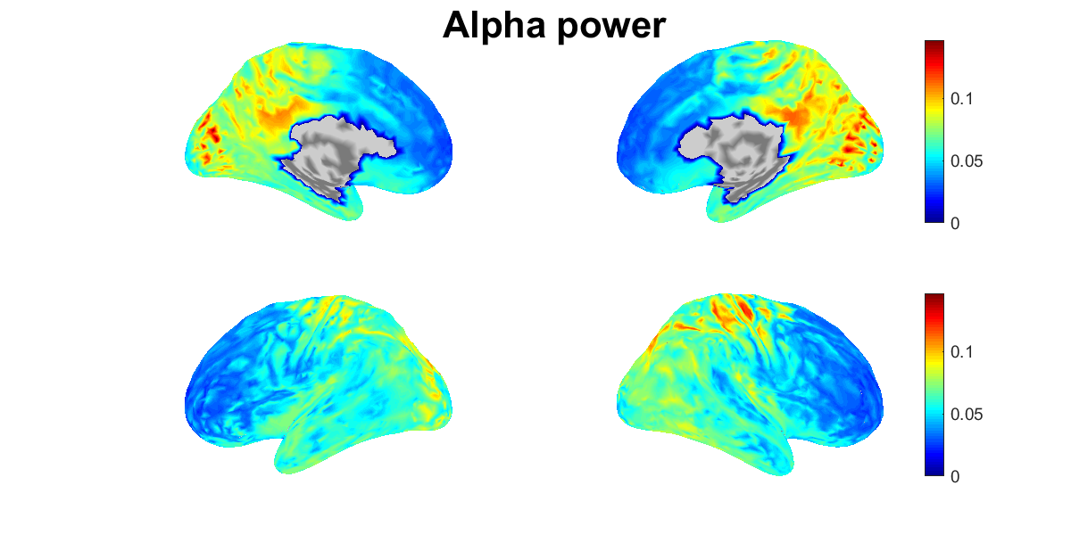
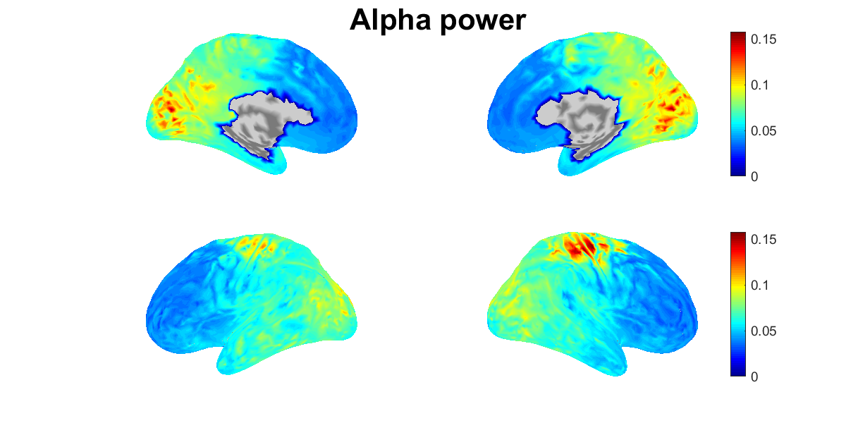
4.9. Showing estimated source current

We show the power spectral densities of the estimated source current. For each vertex, we normalize the current to have mean 0 and standard deviation (SD) 1, and calculate its powers in delta, theta, alpha, beta, and gamma bands. For each band, we show the spatial distributions of the power on the cortex (vb_plot_cortex.m).

Figures will be saved in $your_dir/figure/show_estimated_current_eeg, such as

$your_dir/figure/show_estimated_current_eeg/Alpha_power.png.

5. Source imaging from MEG data

In this section, we introduce the procedures to estimate the source current from the resting-state MEG data.

5.1. Importing MEG data

We convert the Yokogawa MEG files to MAT files (User manual, vb_job_meg.m).

>> import_meg(p);

The following file will be saved.

$your_dir/analyzed_data/MEG/imported/run01.meg.mat

5.2. Removing environmental noise

The MEG data includes large environmental noise from air‐conditioners and others. Using reference sensor data, we remove the environmental noise from the MEG data by time-shift PCA (de Cheveigne and Simon, 2008).

>> denoise_meg(p);

The following file will be saved.

$your_dir/analyzed_data/MEG/denoised/run01.meg.mat

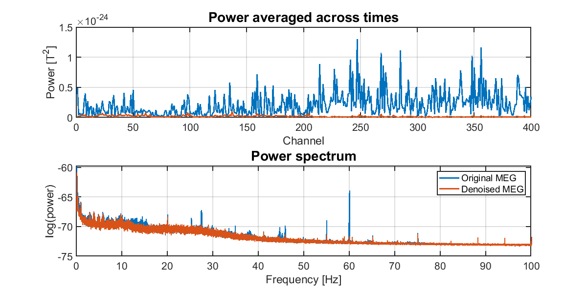
5.3. Checking the result of removing environmental noise

To check whether the environmental noises were appropriately removed, we compare the power spectra between the original and the denoised MEG data.

>> check_denoised_meg(p);

The following figure will be saved.

$your_dir/figure/check_denoised_meg.png

5.4. Filtering MEG data

The MEG data includes drift and line noise (60 Hz at Kansai in Japan). To remove these noises, we apply a low-pass filter, down-sampling, and a high-pass filter.

>> filter_meg(p);

The following file will be saved.

$your_dir/analyzed_data/MEG/filtered/run01.meg.mat

5.5. Preparing leadfield matrix

We make a leadfield matrix, a tranformation matrix from the source current to the MEG data. First, we construct a 1-shell (cerebrospinal fluid) surface model (User manual, vb_job_head_3shell.m). Then, we make the leadfield matrix based on the 1-shell model (User manual, vb_job_leadfield.m).

>> prepare_leadfield_meg(p);

The following files will be saved.

$your_dir/analyzed_data/MEG/leadfield/Subject.head.mat (1-shell model)
$your_dir/analyzed_data/MEG/leadfield/Subject.basis.mat (Leadfield matrix)

5.6. Collecting data

We collect the necessary data for the source imaging (e.g. the MEG data and the leadfield matrix). Hereafter, the data will be saved in a simple format rather than the VBMEG's.

>> collect_data_meg(p);

The following file will be saved.

$your_dir/analyzed_data/MEG/collected/run01.mat

5.7. Removing EOG components

We regress out the EOG components from the MEG data. For each channel, we construct a linear model to predict the MEG data from the EOG data and remove the prediction from the MEG data.

>> remove_eog_meg(p);

The following file will be saved.

$your_dir/analyzed_data/MEG/eog_removed/run01.mat

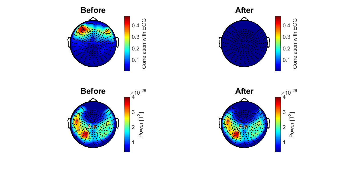
5.8. Checking the result of removing EOG components

To check whether the EOG components were appropriately removed, we calculate the correlation coefficients between the MEG data at each channel and the EOG data. The correlation coefficients are shown on the sensor space (vb_plot_sensor_2d.m).

>> check_eog_removed_meg(p);

The following figure will be saved.

$your_dir/figure/check_eog_removed_meg.png

5.9. Removing bad channels

We remove sleep and noisy channels.

>> remove_bad_ch_meg(p);

The following file will be saved.

$your_dir/analyzed_data/MEG/bad_ch_removed/run01.mat

5.10. Removing ECG components

Using an ICA, we remove ECG components from the MEG data.

>> remove_ecg_by_ica_meg(p);

The following file will be saved.

$your_dir/analyzed_data/MEG/ecg_removed/run01.mat

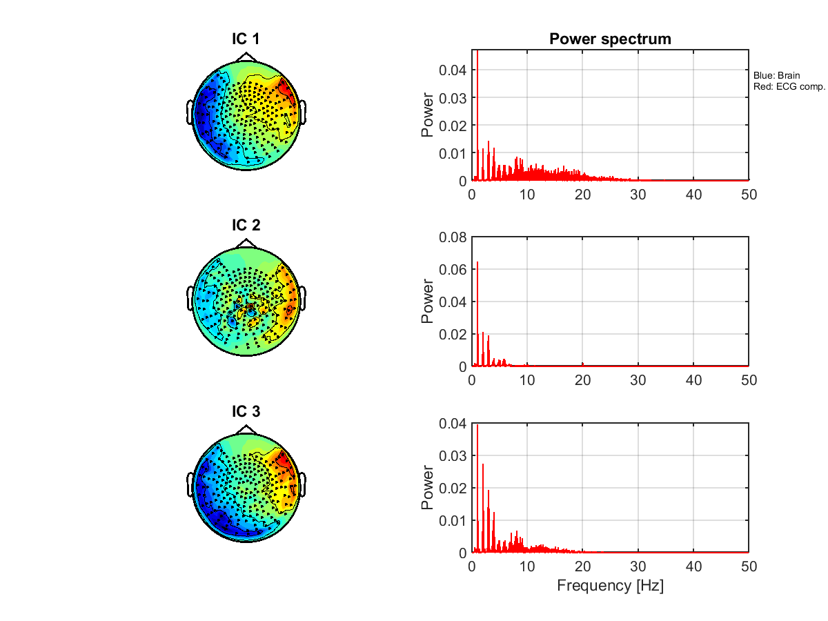
5.11. Showing the ICs

We show the ICs obtained in 5.10. Removing ECG components. The ICs classified as the ECG are indicated by red lines.

Figures will be saved in $your_dir/figure/show_ic_meg, such as

$your_dir/figure/show_ic_meg/1-3.png.

5.12. Estimating source current

We estimate the source current from the preprocessed MEG data by applying the LCMV beamformer.

>> estimate_current_meg(p);

The following file will be saved.

$your_dir/analyzed_data/MEG/source_current/run01.mat

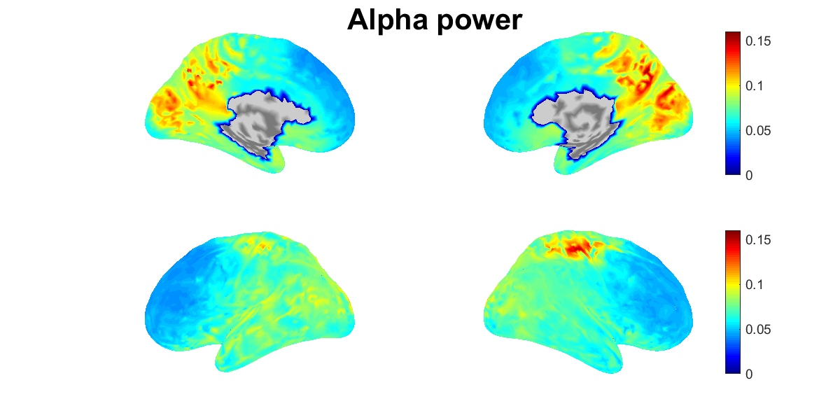
5.13. Showing estimated source current

We show the power spectral densities of the estimated source current. For each vertex, we normalize the current to have mean 0 and SD 1, and calculate its powers in delta, theta, alpha, beta, and gamma bands. For each band, we show the spatial distributions of the power on the cortex (vb_plot_cortex.m).

Figures will be saved in $your_dir/figure/show_estimated_current_meg, such as

$your_dir/figure/show_estimated_current_meg/Alpha_power.png.

6. Source imaging from both EEG and MEG data

In this section, we introduce the procedures to estimate the source current from the resting-state EEG and MEG data.

6.1. Estimating source current

We estimate the source current from the preprocessed EEG and MEG data by applying the LCMV beamformer.

>> estimate_current_meeg(p);

The following file will be saved.

$your_dir/analyzed_data/MEEG/source_current/run01.mat

6.2. Showing estimated source current

We show the power spectral densities of the estimated source current.

Figures will be saved in $your_dir/figure/show_estimated_current_meeg, such as

$your_dir/figure/show_estimated_current_meeg/Alpha_power.png.

emc

Congratulations! You have successfully achieved the goal of this tutorial.

Source imaging from resting-state M/EEG data

Contents

1. Introduction

1.1. Scenario

1.2. Experimental procedure

2. Starting tutorial

2.1. Setting environment

2.2. Adding paths

2.3. Setting parameters

3. Modeling brain

3.1. Importing T1-weighted image

3.2. Correcting bias in T1-weighted image

3.3. Segmenting T1-weighted image

3.4. Constructing cortical surface model from T1-weighted image

3.5. Constructing brain model from the cortical surface model

4. Source imaging from EEG data

4.1. Importing EEG data

4.2. Filtering EEG data

4.3. Preparing leadfield matrix

4.4. Collecting data

4.5. Removing EOG components

4.6. Checking the result of removing EOG components

4.7. Removing bad channels

4.8. Estimating source current

4.9. Showing estimated source current

5. Source imaging from MEG data

5.1. Importing MEG data

5.2. Removing environmental noise

5.3. Checking the result of removing environmental noise

5.4. Filtering MEG data

5.5. Preparing leadfield matrix

5.6. Collecting data

5.7. Removing EOG components

5.8. Checking the result of removing EOG components

5.9. Removing bad channels

5.10. Removing ECG components

5.11. Showing the ICs

5.12. Estimating source current

5.13. Showing estimated source current

6. Source imaging from both EEG and MEG data

6.1. Estimating source current

6.2. Showing estimated source current