MEG source imaging and group analysis

Contents
1. Introduction
2. Starting tutorial
3. Modeling brain
4. Importing fMRI activity
5. MEG source imaging
6. Group analysis
7. EEG source imaging
8. Source imaging from both MEG and EEG data

1. Introduction

1.1. Scenario

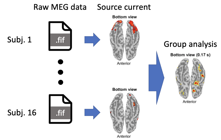
Using VBMEG, we can easily perform a group analysis of source currents estimated from MEG/EEG data. This is because VBMEG defines current sources on individual cortices based on the predefined sources in a standard brain. This allows a simple comparison of the estimated currents across subjects for each source.

Using real experimental data, this tutorial guides through the procedures from importing raw MEG data to a group analysis of source currents. Furthermore, this tutorial demonstrates EEG source imaging. All the procedures will be conducted with scripts.

1.2. Neuromag MEG/EEG data

We use an open MEG/EEG dataset containing 16 subjects' evoked responses to face stimuli (OpenNEURO ds000117-v1.0.1, Wakeman and Henson, 2015).

The Neuromag data can be downloaded also from Amazon S3 by the following command.

$ aws s3 cp --no-sign-request s3://openneuro.org/ds000117 ds000117 --recursive

For installing Amazon Web Service Command Line Interface (AWS CLI), go to its tutorial page.

In their experiment, three types of face stimuli were presented:

Famous,
Unfamiliar,
Scrambled.

During the experiment, MEG and EEG were simultaneously recorded with an Elekta Neuromag Vectorview 306 system (Helsinki, FI). T1 images and fMRIs were also collected with a Siemens 3T TIM TRIO (Siemens, Erlangen, Germany).

2. Starting tutorial

2.1. Setting environment

This tutorial was developed using MATLAB 2019a with Signal Processing Toolbox on Linux.

(1) Download and put the Neuromag MEG data into $data_dir
(2) Download, unzip, and put tutorial.zip into $your_dir
(5) Start MATLAB and change current directory to $your_dir/program
(6) Open make_all.m by typing

>> open make_all

2.2. Adding necessary toolboxes to search path

Thereafter, we will sequentially execute the commands in make_all.m from the top.

We set directories of necessary toolboxes: VBMEG and SPM8. Please modify these for your environment.

>> path_of_VBMEG = '/home/cbi/takeda/analysis/toolbox/vbmeg_20220721';
>> path_of_SPM8 = '/home/cbi-data20/common/software/external/spm/spm8';

We add the toolboxes to search path.

>> addpath(path_of_VBMEG);
>> vbmeg
>> addpath(path_of_SPM8);

2.3. Setting parameters

We set the parameters for analyzing the MEG data, and set the file and directory names.

>> data_root = $data_dir;
>> sub_number = 1;
>> p = set_parameters(data_root, sub_number);

By default, analyzed data and figures will be respectively saved in

$your_dir/analyzed_data/sub-01,
$your_dir/figure.

3. Modeling brain

First of all, we construct a cortical surface model from the T1 image and define current sources on it.

3.1. Importing T1 image

We unzip the T1 image, and convert its coordinate system to those of VBMEG (direction: RAS, origin: center of T1 image). The coordinates of fiducials are also converted.

>> import_T1(p)

The following files will be saved.

$your_dir/analyzed_data/sub-01/struct/Subject.nii (converted T1 image)
$your_dir/analyzed_data/sub-01/struct/fiducial.mat (converted coordinates of fiducials)

3.2. Correcting bias in T1 image

Using SPM8, we correct bias in the T1 image (User manual).

>> correct_bias_in_T1(p)

The following file will be saved.

$your_dir/analyzed_data/sub-01/struct/mSubject.nii

3.3. Segmenting T1 image

Using SPM8, we extract a gray matter image from the T1 image.

>> segment_T1(p)

The following files will be saved.

$your_dir/analyzed_data/sub-01/struct/c1mSubject.nii (Gray matter)
$your_dir/analyzed_data/sub-01/struct/mSubject_seg_sn.mat (Normalization)

The gray matter image will be used in 5.2.1. Preparing leadfield, and the normalization file will be used in 4. Importing fMRI activity.

3.4. Constructing brain model from cortical surface model

Using FreeSurfer, we constructed a polygon model of a cortical surface from the T1 image (User manual). By importing the cortical surface model, we construct a brain model, in which current sources are defined (vb_job_brain.m).

>> construct_brain_model(p)

The following files will be saved.

$your_dir/analyzed_data/sub-01/brain/Subject.brain.mat (Brain model)
$your_dir/analyzed_data/sub-01/brain/Subject.act.mat

In Subject.act.mat, fMRI activity will be stored (4. Importing fMRI activity).

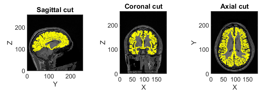
3.5 Checking brain model

We check the constructed brain model by plotting the current sources on the T1 image.

>> check_brain_model(p)

The following figure will be saved.

$your_dir/figure/check_brain_model/sub-01.png

4. Importing fMRI activity

VBMEG estimates source currents from EEG/MEG data using fMRI activity as prior information on the source current variance distribution. The fMRI result is assumed to be obtained using SPM8 (User manual).

4.1. Importing fMRI activity

We import the statistical results of the fMRI data (SPM.mat, vb_job_fmri.m).

>> import_fmri(p)

T-values and percent signal changes will be stored in

$your_dir/analyzed_data/sub-01/brain/Subject.act.mat.

4.2. Checking imported fMRI activity

We check the imported fMRI activities (vb_plot_cortex.m).

>> check_imported_fmri(p)

The following figure will be saved.

$your_dir/figure/check_imported_fmri/sub-01/2.png

5. MEG source imaging

In this section, we estimate source currents from the MEG data. If you are only interested in EEG source imaging, you can skip this section to 7. EEG source imaging.

5.1. Preprocessing MEG data

We import the Neuromag MEG data (.fif) and preprocess them for source imaging.

5.1.1. Importing MEG data

We convert the Neuromag MEG files (.fif) into the VBMEG format (.meg.mat) (User manual) while converting the sensor positions into the VBMEG coordinate system (direction: RAS, origin: center of T1 image).

>> import_meg(p)

The imported MEG data will be saved in

$your_dir/analyzed_data/sub-01/meg/imported.

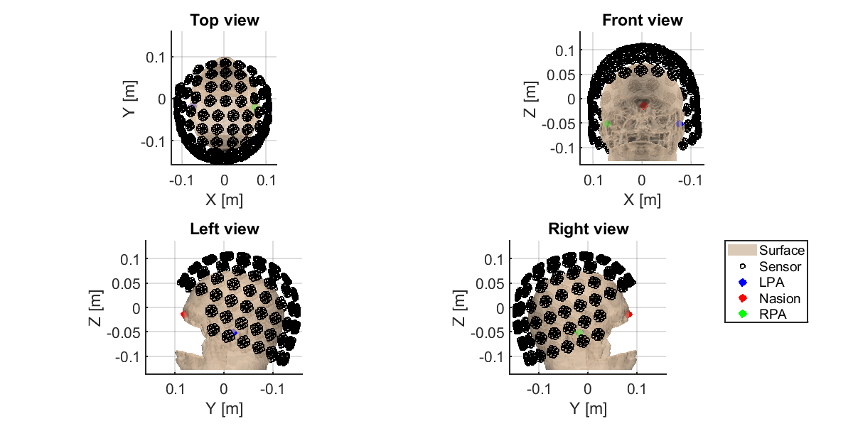
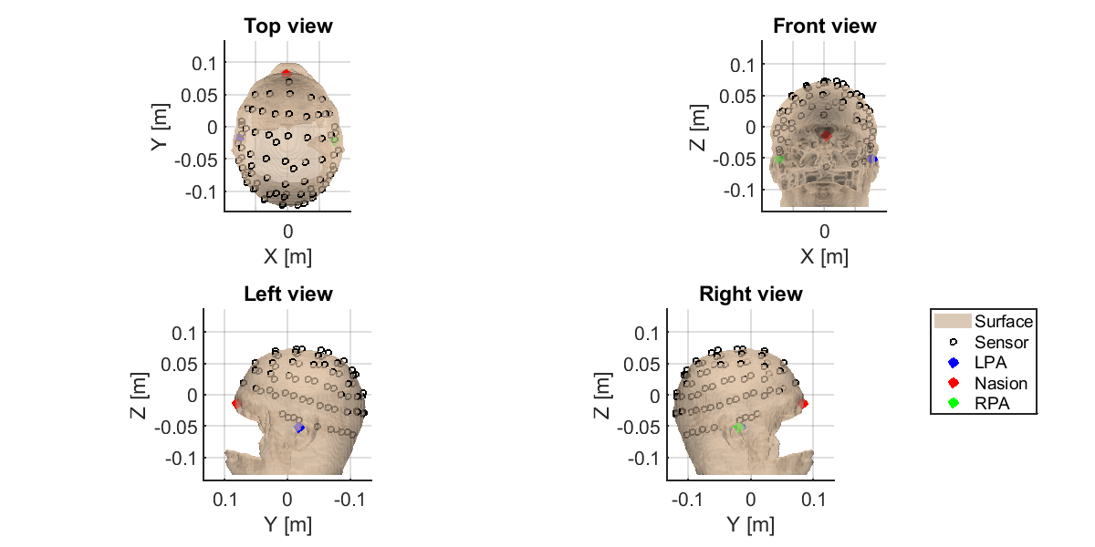
5.1.2. Checking sensor positions

We check the converted sensor positions by showing them with the head surface extracted from the T1 image.

>> check_pos_meg(p)

The following figure will be saved.

$your_dir/figure/check_pos_meg/sub-01/Sensor.png

5.1.3. Denoising MEG data

The MEG data include such environmental noises as line and biological noises from eye movements and heartbeats. To remove them, we apply a low-pass filter, down-sampling, and a high-pass filter, and regress out ECG and EOG components

>> denoise_meg(p)

The denoised MEG data will be saved in

$your_dir/analyzed_data/sub-01/meg/denoised.

5.1.4. Making trial data

We segment the continuous MEG data into trials. First, we detect stimulus onsets from the trigger signals. Then, we segment the MEG data into trials by the detected stimulus onsets.

>> make_trial_meg(p)

The following files will be saved.

$your_dir/analyzed_data/sub-01/meg/trial/run-{01-06}.meg.mat

5.1.5. Correcting baseline

For each channel and trial, we make the average of prestimulus MEG to 0.

>> correct_baseline_meg(p)

The following files will be saved.

$your_dir/analyzed_data/sub-01/meg/trial/brun-{01-06}.meg.mat

5.1.6. Combining trials across runs

To handle all the trials collectively, we virtually combine the trials across all the runs.

>> combine_trial_meg(p)

The following file will be saved.

$your_dir/analyzed_data/sub-01/meg/trial/All.info.mat

This file contains the information (e.g. file paths) to serve as the shortcut to these files.

$your_dir/analyzed_data/sub-01/meg/trial/brun-{01-06}.meg.mat

5.1.7. Rejecting bad channels

We detect noisy channels based on the amplitudes of the MEG data and reject them. The rejected channels will not be used in the following analyses.

>> reject_channel_meg(p)

The following file will be saved.

$your_dir/analyzed_data/sub-01/meg/trial/cAll.info.mat

5.1.8. Rejecting bad trials

We reject the trials in which the subject blinked during the exposure to the visual stimuli. The rejected trials will not be used in the following analyses.

>> reject_trial_meg(p)

The following file will be saved.

$your_dir/analyzed_data/sub-01/meg/trial/tcAll.info.mat

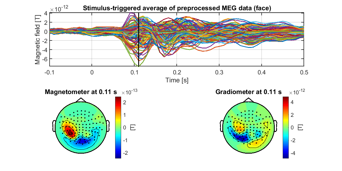
5.1.9. Showing preprocessed MEG data

For each condition, we show the processed MEG data averaged across the trials (vb_plot_sensor_2d.m).

>> show_preprocessed_meg(p)

The following figure will be saved.

$your_dir/figure/show_preprocessed_meg/sub-01/Face.png

5.2. Estimating source current from MEG data

5.2.1. Preparing leadfield

First, we construct a 1-shell (cerebrospinal fluid) head conductivity model for MEG source imaging (User manual, vb_job_head_3shell.m). Then, we make the leadfield matrix based on the head conductivity model (User manual, vb_job_leadfield.m).

>> prepare_leadfield_meg(p)

The following files will be saved.

$your_dir/analyzed_data/sub-01/meg/leadfield/Subject.head.mat (1-shell head conductivity model)
$your_dir/analyzed_data/sub-01/meg/leadfield/Subject.basis.mat (Leadfield matrix)

5.2.2. Estimating source currents

First, we estimate the current variance by integrating the fMRI activity and the MEG data (User manual, vb_job_vb.m). Then, we estimate source currents using the current variance (User manual, vb_job_current.m].

>> estimate_source_current_meg(p)

The following files will be saved.

$your_dir/analyzed_data/sub-01/meg/current/tcAll.bayes.mat (Current variance)
$your_dir/analyzed_data/sub-01/meg/current/tcAll.curr.mat (Source current)

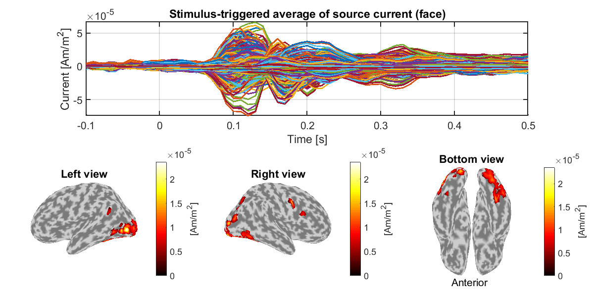
5.2.3. Showing estimated source currents

For each condition, we show the estimated source currents averaged across the trials (vb_plot_cortex.m).

>> show_source_current_meg(p)

The following figure will be saved.

$your_dir/figure/show_source_current_meg/sub-01/Face.png

6. Group analysis

In this section, we perform a group analysis using all the subjects' source currents estimated from the MEG data.

6.1. Comparing current amplitudes between conditions

For each vertex and time, we compare the current amplitudes between the face (famous and unfamiliar) and scrambled conditions. This is the multiple comparison problem, which we solve by controlling the false discovery rate (FDR). The FDRs are estimated by the method of Storey and Tibshrani, 2003.

>> examine_diff_between_conds(p)

The results will be saved in

$your_dir/analyzed_data/group/examine_diff_between_conds.

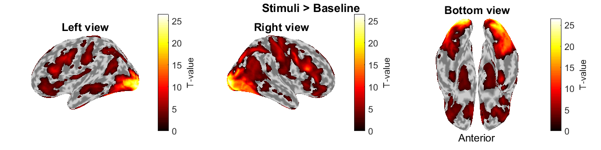
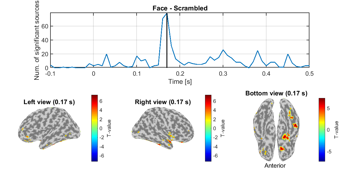
6.2. Showing differences of current amplitudes across conditions

We show the significant differences of the current amplitudes.

>> show_diff_between_conds(p)

The following figure will be saved.

$your_dir/figure/show_diff_between_conds/Face-Scrambled.png

7. EEG source imaging

In this section, we estimate source currents from the EEG data.

7.1. Preprocessing EEG data

We import the Neuromag EEG data (.fif) and preprocess them for source imaging.

7.1.1. Importing EEG data

We convert the Neuromag EEG files (.fif) into the VBMEG format (.meg/eeg.mat) (User manual) while converting the sensor positions into the VBMEG coordinate system (direction: RAS, origin: center of T1 image).

>> import_eeg(p)

The imported EEG data will be saved in

$tutorial_dir/result/sub-01/eeg/imported.

7.1.2. Checking sensor positions

We check the converted sensor positions by showing them with the head surface extracted from the T1 image.

>> check_pos_eeg(p)

The following figure will be saved.

$tutorial_dir/result/figure/check_pos_eeg/sub-01/Sensor.png

7.1.3. Denoising EEG data

The EEG data include environmental and biological noises. To remove them, we apply a low-pass filter, down-sampling, and a high-pass filter, and regress out ECG and EOG components

>> denoise_eeg(p)

The denoised EEG data will be saved in

$tutorial_dir/result/sub-01/eeg/denoised.

7.1.4. Making trial data

We segment the continuous EEG data into trials. First, we detect stimulus onsets from the trigger signals. Then, we segment the EEG data into trials by the detected stimulus onsets.

>> make_trial_eeg(p)

The following files will be saved.

$tutorial_dir/result/sub-01/eeg/trial/run-{01-06}.eeg.mat

7.1.5. Correcting baseline

For each channel and trial, we make the average of prestimulus EEG to 0.

>> correct_baseline_eeg(p)

The following files will be saved.

$tutorial_dir/result/sub-01/eeg/trial/brun-{01-06}.eeg.mat

7.1.6. Combining trials across runs

To handle all the trials collectively, we virtually combine the trials across all the runs.

>> combine_trial_eeg(p)

The following file will be saved.

$tutorial_dir/result/sub-01/eeg/trial/All.info.mat

This file contains the information (e.g. file paths) to serve as the shortcut to these files.

$tutorial_dir/result/sub-01/eeg/trial/brun-{01-06}.eeg.mat

7.1.7. Rejecting bad channels

We detect noisy channels based on the amplitudes of the EEG data and reject them. The rejected channels will not be used in the following analyses.

>> reject_channel_eeg(p)

The following file will be saved.

$tutorial_dir/result/sub-01/eeg/trial/cAll.info.mat

7.1.8. Rejecting bad trials

We reject the trials in which the subject blinked during the exposure to the visual stimuli. The rejected trials will not be used in the following analyses.

>> reject_trial_eeg(p)

The following file will be saved.

$tutorial_dir/result/sub-01/eeg/trial/tcAll.info.mat

7.1.9. Taking common average reference

We take a common average reference; that is, we make the averages of EEG data across the channels to 0.

>> take_common_average_eeg(p)

The following files will be saved.

$tutorial_dir/result/sub-01/eeg/trial/ctcAll.info.mat (Shortcut to the following files)
$tutorial_dir/result/sub-01/eeg/trial/cbrun-{01-06}.eeg.mat

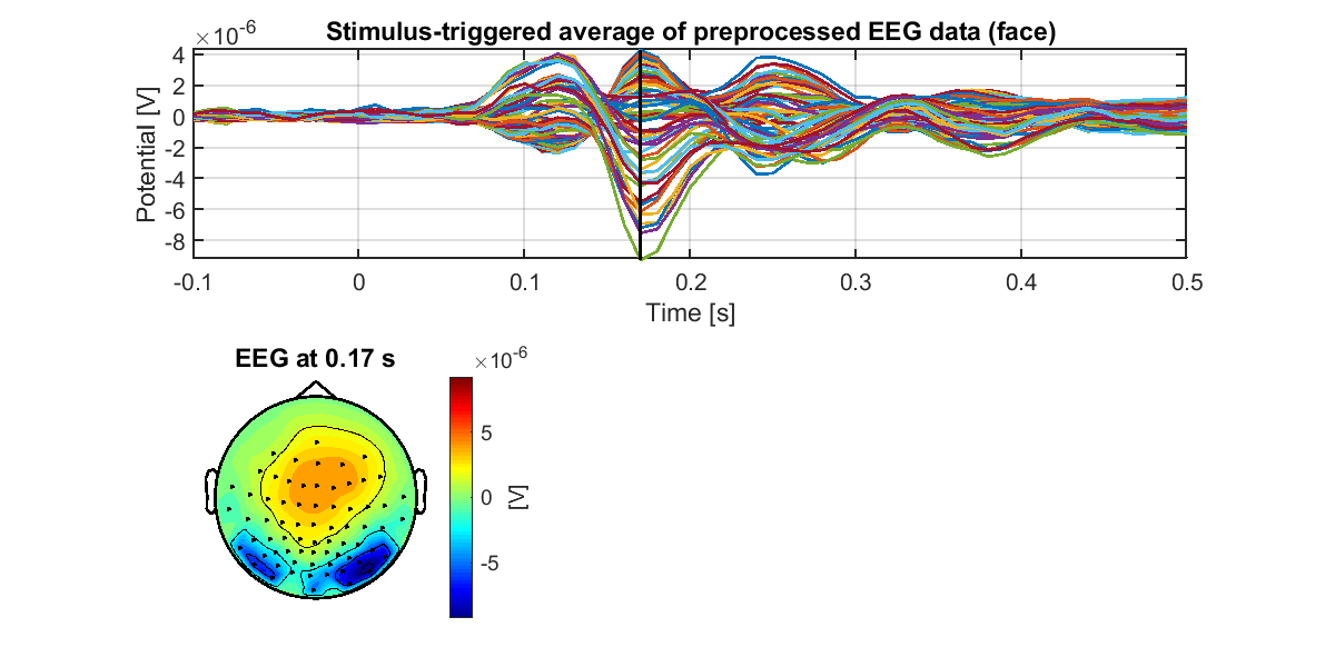
7.1.10. Showing preprocessed EEG data

For each condition, we show the processed EEG data averaged across the trials (vb_plot_sensor_2d.m).

>> show_preprocessed_eeg(p)

The following figure will be saved.

$tutorial_dir/result/figure/show_preprocessed_eeg/sub-01/Face.png

7.2. Estimating source current from EEG data

We estimate source currents from the preprocessed EEG data.

7.2.1. Preparing leadfield

First, we construct a 3-shell (cerebrospinal fluid, skull, and scalp) head conductivity model for EEG source imaging (User manual, vb_job_head_3shell.m). Then, we make the leadfield matrix based on the head conductivity model (User manual, vb_job_leadfield.m).

>> prepare_leadfield_eeg(p)

The following files will be saved.

$tutorial_dir/result/sub-01/eeg/leadfield/Subject.head.mat (3-shell head conductivity model)
$tutorial_dir/result/sub-01/eeg/leadfield/Subject.basis.mat (Leadfield matrix)

7.2.2. Estimating source currents

First, we estimate the current variance by integrating the fMRI activity and the EEG data (User manual, vb_job_vb.m). Then, we estimate source currents using the current variance (User manual, vb_job_current.m).

>> estimate_source_current_eeg(p)

The following files will be saved.

$tutorial_dir/result/sub-01/eeg/current/ctcAll.bayes.mat (Current variance)
$tutorial_dir/result/sub-01/eeg/current/ctcAll.curr.mat (Source current)

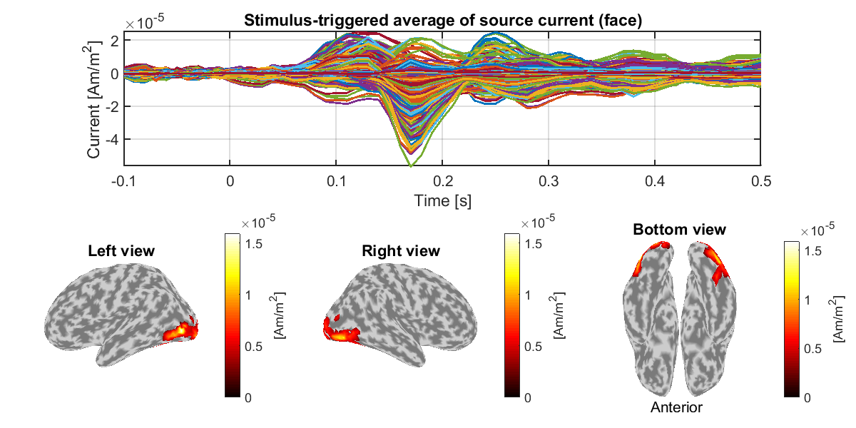
7.2.3. Showing estimated source currents

For each condition, we show the estimated source currents averaged across the trials (vb_plot_cortex.m).

>> show_source_current_eeg(p)

The following figure will be saved.

$tutorial_dir/result/figure/show_source_current_eeg/sub-01/Face.png

8. Source imaging from both MEG and EEG data

In this section, we estimate source currents from both MEG and EEG data.

8.1. Matching trials between MEG and EEG

We match the trials between the MEG and EEG data so that identical trials remain.

>> match_trial_meeg(p)

The following files will be saved.

$tutorial_dir/result/sub-01/meg/trial/mtcAll.info.mat
$tutorial_dir/result/sub-01/eeg/trial/mctcAll.info.mat

8.2. Estimating source currents

First, we estimate the current variance by integrating the fMRI activity, the MEG, and the EEG data (User manual, vb_job_vb.m]). Then, we estimate source currents using the current variance (User manual, vb_job_current.m).

>> estimate_source_current_meeg(p)

The following files will be saved.

$tutorial_dir/result/sub-01/meeg/current/mtcAll.bayes.mat (Current variance)
$tutorial_dir/result/sub-01/meeg/current/mtcAll.curr.mat (Source current)

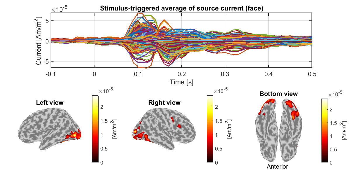
8.3. Showing estimated source currents

For each condition, we show the estimated source currents averaged across the trials (vb_plot_cortex.m).

>> show_source_current_meeg(p)

The following figure will be saved.

$tutorial_dir/result/figure/show_source_current_meeg/sub-01/Face.png

mec

Congratulations! You have successfully achieved the goal of this tutorial.

MEG source imaging and group analysis

Contents

1. Introduction

1.1. Scenario

1.2. Neuromag MEG/EEG data

2. Starting tutorial

2.1. Setting environment

2.2. Adding necessary toolboxes to search path

2.3. Setting parameters

3. Modeling brain

3.1. Importing T1 image

3.2. Correcting bias in T1 image

3.3. Segmenting T1 image

3.4. Constructing brain model from cortical surface model

3.5 Checking brain model

4. Importing fMRI activity

4.1. Importing fMRI activity

4.2. Checking imported fMRI activity

5. MEG source imaging

5.1. Preprocessing MEG data

5.1.1. Importing MEG data

5.1.2. Checking sensor positions

5.1.3. Denoising MEG data

5.1.4. Making trial data

5.1.5. Correcting baseline

5.1.6. Combining trials across runs

5.1.7. Rejecting bad channels

5.1.8. Rejecting bad trials

5.1.9. Showing preprocessed MEG data

5.2. Estimating source current from MEG data

5.2.1. Preparing leadfield

5.2.2. Estimating source currents

5.2.3. Showing estimated source currents

6. Group analysis

6.1. Comparing current amplitudes between conditions

6.2. Showing differences of current amplitudes across conditions

7. EEG source imaging

7.1. Preprocessing EEG data

7.1.1. Importing EEG data

7.1.2. Checking sensor positions

7.1.3. Denoising EEG data

7.1.4. Making trial data

7.1.5. Correcting baseline

7.1.6. Combining trials across runs

7.1.7. Rejecting bad channels

7.1.8. Rejecting bad trials

7.1.9. Taking common average reference

7.1.10. Showing preprocessed EEG data

7.2. Estimating source current from EEG data

7.2.1. Preparing leadfield

7.2.2. Estimating source currents

7.2.3. Showing estimated source currents

8. Source imaging from both MEG and EEG data

8.1. Matching trials between MEG and EEG

8.2. Estimating source currents

8.3. Showing estimated source currents