Neuromag tutorial
Contents
- Contents
- 0. Download
- 1. Introduction
- 2. Starting tutorial
- 3. Modeling brain
- 4. Importing fMRI activity
- 5. MEG source imaging
- 6. Group analysis
- 7. Comparing with other source imaging methods
- 8. EEG source imaging
- 9. Connectome dynamics estimation
0. Download
- Neuromag MEG/EEG data (OpenNEURO ds000117-v1.0.1, Wakeman and Henson, 2015)
- Tutorial programs, FreeSurfer results, and fMRI activities (tutorial.zip)
The same Neuromag data can be downloaded also from Amazon S3 by the following command.
$ aws s3 cp --no-sign-request s3://openneuro.org/ds000117 ds000117 --recursive
For installing Amazon Web Service Command Line Interface (AWS CLI), go to its tutorial page.
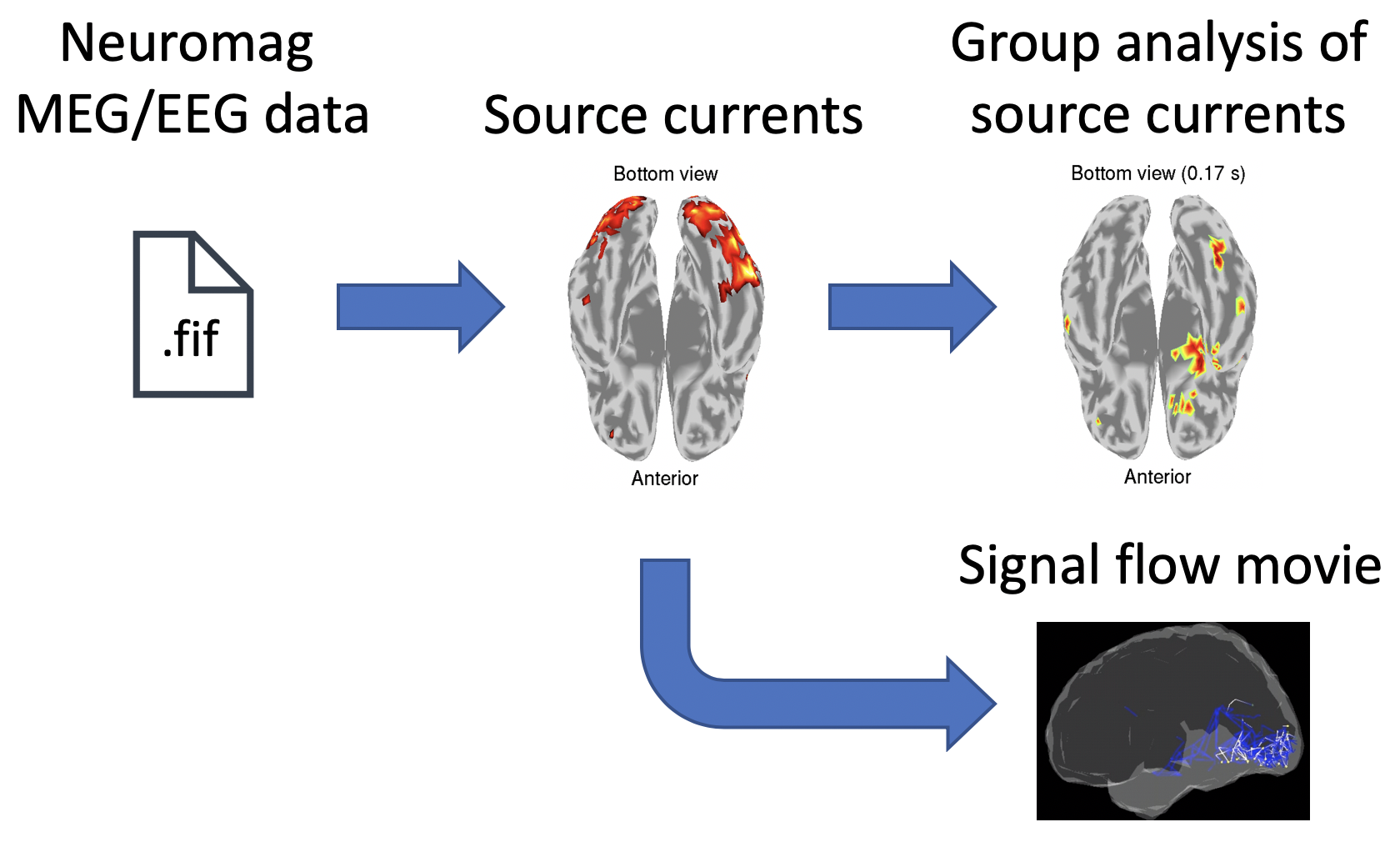
1. Introduction
1.1. Scenario
VBMEG can import MEG data recorded by Elekta Neuromag as well as Yokogawa system. By collaborating with VBMEG's tutorial paper, this page guides through the procedure from importing Neuromag MEG/EEG data to a group analyses of source currents and a connectome dynamics estimation. The estimated connectome dynamics will be shown by a movie displaying signal flows between brain regions. All the procedures will be conducted with scripts.
1.2. Neuromag MEG/EEG data
We use an open MEG/EEG dataset containing 16 subjects' evoked responses to face stimuli (OpenNEURO ds000117-v1.0.1, Wakeman and Henson, 2015). In their experiment, three types of face stimuli were presented:
- Famous,
- Unfamiliar,
- Scrambled.
During the experiment, MEG and EEG were simultaneously recorded with an Elekta Neuromag Vectorview 306 system (Helsinki, FI). T1 images and fMRIs were also collected with a Siemens 3T TIM TRIO (Siemens, Erlangen, Germany).
2. Starting tutorial
2.1. Setting environment
This tutorial was developed using MATLAB 2018b with Signal Processing Toolbox on Linux. To proceed to the connectome dynamics estimation, FSL and MRtrix need to be installed for dMRI processing (required environment for dMRI processing) and "vbmegrc" under the VBMEG directory needs to be modified for your environment.
(1) Download and put the Neuromag MEG/EEG data into $data_dir
(2) Download, unzip, and put the tutorial programs and prepared results into $tutorial_dir
(5) Start MATLAB and change current directory to $tutorial_dir/program
(6) Open make_all.m by typing
>> open make_all
2.2. Adding path
Thereafter, we will sequentially execute the commands in make_all.m from the top.
We add paths to necessary directories.
>> addpath(path_of_VBMEG)
>> vbmeg
>> addpath(path_of_SPM8)
>> addpath('common')
You need to modify path_of_VBMEG and path_of_SPM8 for your environment.
2.3. Creating project
We set the file and directory names, and set the parameters for analyzing the data.
>> data_root = $data_dir;
>> tutorial_root = $tutorial_dir;
>> sub_number = 1;
>> p = create_project(data_root, tutorial_root, sub_number);
Results will be saved in $tutorial_dir/result.
3. Modeling brain
First of all, we construct a cortical surface model from the T1 image and define current sources on it.
3.1. Importing T1 image
We unzip the T1 image, and convert its coordinate system to those of VBMEG (direction: RAS, origin: center of T1 image). The coordinates of fiducials are also converted.
>> import_T1(p)
The following files will be saved.
- $tutorial_dir/result/sub-01/struct/Subject.nii (converted T1 image)
- $tutorial_dir/result/sub-01/struct/fiducial.mat (converted coordinates of fiducials)
3.2. Correcting bias in T1 image
Using SPM8, we correct bias in the T1 image (User manual).
>> correct_bias_in_T1(p)
The following file will be saved.
- $tutorial_dir/result/sub-01/struct/mSubject.nii
3.3. Segmenting T1 image
Using SPM8, we extract a gray matter image from the T1 image.
>> segment_T1(p)
The following files will be saved.
- $tutorial_dir/result/sub-01/struct/c1mSubject.nii (Gray matter)
- $tutorial_dir/result/sub-01/struct/mSubject_seg_sn.mat (Normalization)
The gray matter image will be used in 5.2.1. Preparing leadfield, and the normalization file will be used in 4. Importing fMRI activity.
3.4. Constructing brain model from cortical surface model
Using FreeSurfer, we constructed a polygon model of a cortical surface from the T1 image (User manual). By importing the cortical surface model, we construct a brain model, in which current sources are defined (vb_job_brain.m).
>> construct_brain_model(p)
The following files will be saved.
- $tutorial_dir/result/sub-01/brain/Subject.brain.mat (Brain model)
- $tutorial_dir/result/sub-01/brain/Subject.act.mat
In Subject.act.mat, fMRI activity will be stored (4. Importing fMRI activity).
3.5 Checking brain model
We check the constructed brain model by plotting the current sources on the T1 image.
>> check_brain_model(p)
The following figure will be saved.
- $tutorial_dir/result/figure/check_brain_model/sub-01.png
4. Importing fMRI activity
VBMEG estimates source currents from EEG/MEG data using fMRI activity as prior information on the source current variance distribution. The fMRI result is assumed to be obtained using SPM8 (User manual, vb_job_fmri.m).
4.1. Importing fMRI activity
We import the statistical results of the fMRI data (SPM.mat).
>> import_fmri(p)
T-values and percent signal changes will be stored in
- $tutorial_dir/result/sub-01/brain/Subject.act.mat.
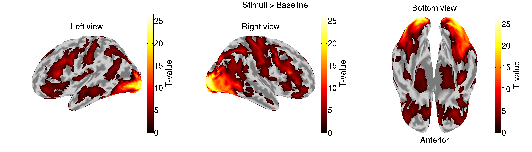
4.2. Checking imported fMRI activity
We check the imported fMRI activities (vb_plot_cortex.m).
>> check_imported_fmri(p)
The following figure will be saved.
5. MEG source imaging
In this section, we estimate source currents from the Neuromag MEG data.
5.1. Preprocessing MEG data
We import the Neuromag MEG data (.fif) and preprocess them for source imaging.
5.1.1. Importing MEG data
We convert the Neuromag MEG files (.fif) into the VBMEG format (.meg.mat) (User manual, vb_job_meg.m) while converting the sensor positions into the VBMEG coordinate system (direction: RAS, origin: center of T1 image).
>> import_meg(p)
The imported MEG data will be saved in
- $tutorial_dir/result/sub-01/meg/imported.
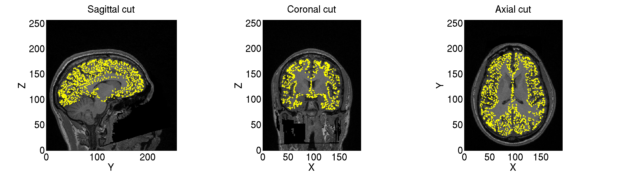
5.1.2. Checking sensor positions
We check the converted sensor positions by showing them with the head surface extracted from the T1 image.
>> check_pos_meg(p)
The following figure will be saved.
- $tutorial_dir/result/figure/check_pos_meg/sub-01/Sensor.png
5.1.3. Denoising MEG data
The MEG data include such environmental noises as line and biological noises from eye movements and heartbeats. To remove them, we apply a low-pass filter, down-sampling, and a high-pass filter, and regress out ECG and EOG components
>> denoise_meg(p)
The denoised MEG data will be saved in
- $tutorial_dir/result/sub-01/meg/denoised.
5.1.4. Making trial data
We segment the continuous MEG data into trials. First, we detect stimulus onsets from the trigger signals. Then, we segment the MEG data into trials by the detected stimulus onsets.
>> make_trial_meg(p)
The following files will be saved.
- $tutorial_dir/result/sub-01/meg/trial/run-{01-06}.meg.mat
5.1.5. Correcting baseline
For each channel and trial, we make the average of prestimulus MEG to 0.
>> correct_baseline_meg(p)
The following files will be saved.
- $tutorial_dir/result/sub-01/meg/trial/brun-{01-06}.meg.mat
5.1.6. Combining trials across runs
To handle all the trials collectively, we virtually combine the trials across all the runs.
>> combine_trial_meg(p)
The following file will be saved.
- $tutorial_dir/result/sub-01/meg/trial/All.info.mat
This file contains the information (e.g. file paths) to serve as the shortcut to these files.
- $tutorial_dir/result/sub-01/meg/trial/brun-{01-06}.meg.mat
5.1.7. Rejecting bad channels
We detect noisy channels based on the amplitudes of the MEG data and reject them. The rejected channels will not be used in the following analyses.
>> reject_channel_meg(p)
The following file will be saved.
- $tutorial_dir/result/sub-01/meg/trial/cAll.info.mat
5.1.8. Rejecting bad trials
We reject the trials in which the subject blinked during the exposure to the visual stimuli. The rejected trials will not be used in the following analyses.
>> reject_trial_meg(p)
The following file will be saved.
- $tutorial_dir/result/sub-01/meg/trial/tcAll.info.mat
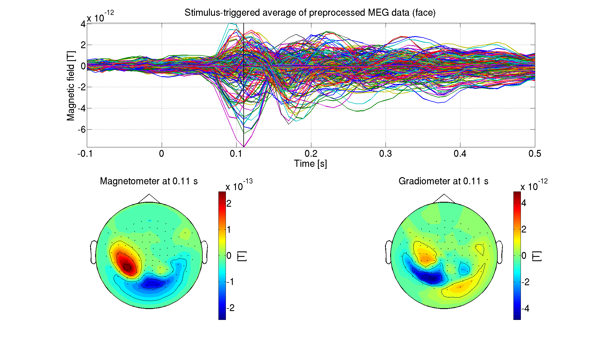
5.1.9. Showing preprocessed MEG data
For each condition, we show the processed MEG data averaged across the trials (vb_plot_sensor_2d.m).
>> show_preprocessed_meg(p)
The following figure will be saved.
- $tutorial_dir/result/figure/show_preprocessed_meg/sub-01/Face.png
5.2. Estimating source current from MEG data
5.2.1. Preparing leadfield
First, we construct a 1-shell (cerebrospinal fluid) head conductivity model for MEG source imaging (User manual, vb_job_head_3shell.m). Then, we make the leadfield matrix based on the head conductivity model (User manual, vb_job_leadfield.m).
>> prepare_leadfield_meg(p)
The following files will be saved.
- $tutorial_dir/result/sub-01/meg/leadfield/Subject.head.mat (1-shell head conductivity model)
- $tutorial_dir/result/sub-01/meg/leadfield/Subject.basis.mat (Leadfield matrix)
5.2.2. Estimating source currents
First, we estimate the current variance by integrating the fMRI activity and the MEG data (User manual, vb_job_vb.m). Then, we estimate source currents using the current variance (User manual, vb_job_current.m).
>> estimate_source_current_meg(p)
The following files will be saved.
- $tutorial_dir/result/sub-01/meg/current/tcAll.bayes.mat (Current variance)
- $tutorial_dir/result/sub-01/meg/current/tcAll.curr.mat (Source current)
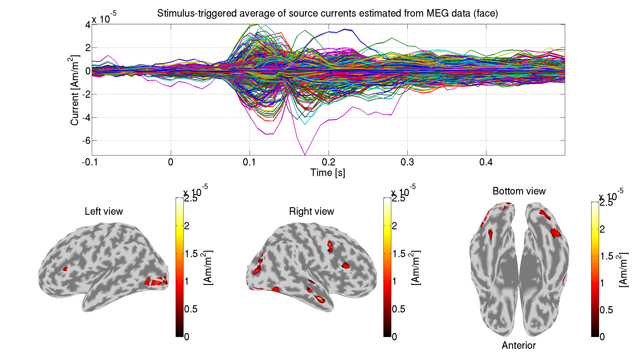
5.2.3. Showing estimated source currents
For each condition, we show the estimated source currents averaged across the trials (vb_plot_cortex.m).
>> show_source_current_meg(p)
The following figure will be saved.
- $tutorial_dir/result/figure/show_source_current_meg/sub-01/Face.png
6. Group analysis
In this section, we perform a group analysis using all the subjects' source currents estimated from the MEG data.
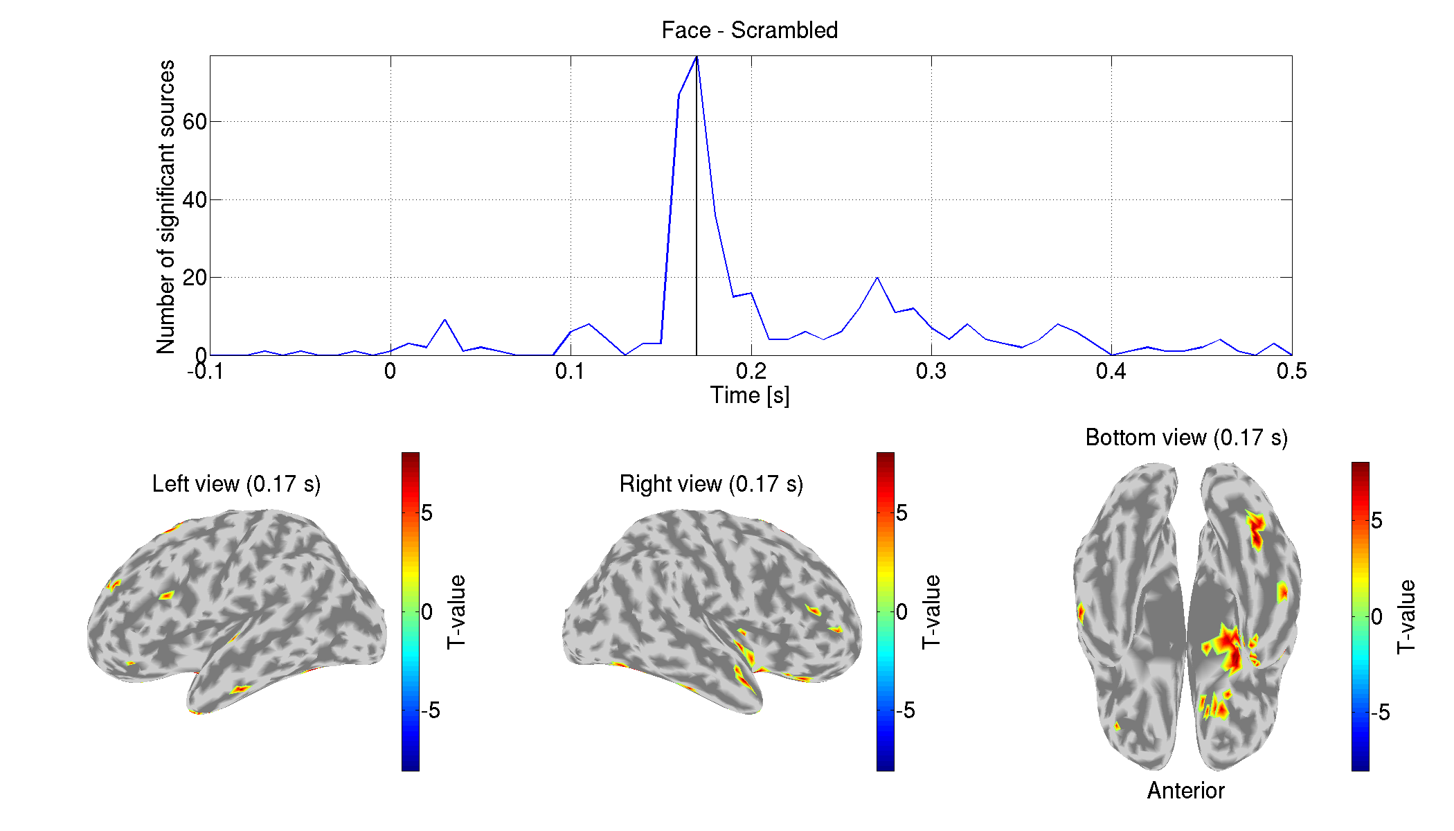
6.1. Comparing current amplitudes between conditions
For each vertex and time, we compare the current amplitudes between the face (famous and unfamiliar) and scrambled conditions. This is the multiple comparison problem, which we solve by controlling the false discovery rate (FDR). The FDRs are estimated by the method of Storey and Tibshrani, 2003.
>> examine_diff_between_conds(p)
The results will be saved in
- $tutorial_dir/result/group/examine_diff_between_conds.
6.2. Showing differences of current amplitudes across conditions
We show the significant differences of the current amplitudes.
>> show_diff_between_conds(p)
The following figure will be saved.
- $tutorial_dir/result/figure/show_diff_between_conds/Face-Scrambled.png
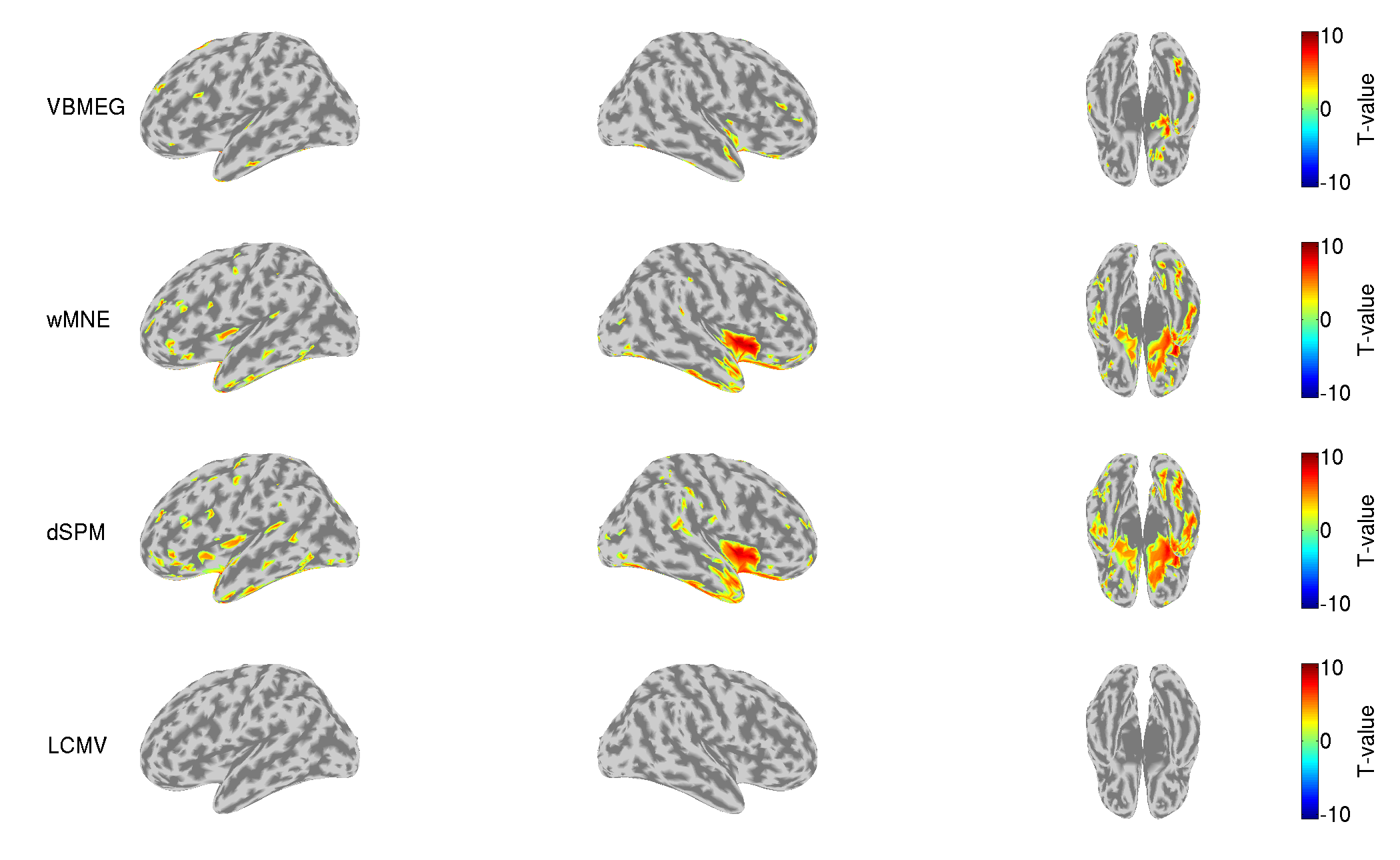
7. Comparing with other source imaging methods
In this section, we compare the above results with those estimated using other source imaging methods: weighted Minimum Norm Estimate (wMNE), dynamic Statistical Parametric Mapping (dSPM), and Linearly Constrained Minimum Variance (LCMV) beamformer. They will be performed using Brainstorm functions.
>> addpath(genpath(path_of_Brainstorm))
>> addpath('compare_with_other_methods')
>> make_all_bst
>> rmpath(genpath(path_of_Brainstorm))
You need to modify path_of_Brainstorm for your environment.
The following figures will be saved.
- $tutorial_dir/result/figure/show_source_current_comparison/sub-01.png
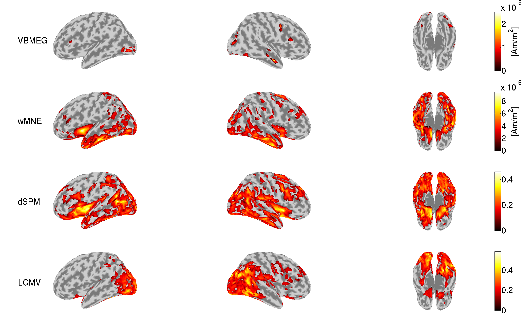
- $tutorial_dir/result/figure/show_diff_between_conds_comparison/Face-Scrambled.png
8. EEG source imaging
In this section, we estimate source currents from the Neuromag EEG data.
8.1. Creating project
We set the file and directory names.
>> sub_number = 1;
>> p = create_project(data_root, tutorial_root, sub_number);
8.2. Preprocessing EEG data
We import the Neuromag EEG data (.fif) and preprocess them for source imaging.
8.2.1. Importing EEG data
We convert the Neuromag EEG files (.fif) into the VBMEG format (.meg/eeg.mat) (User manual, vb_job_meg.m) while converting the sensor positions into the VBMEG coordinate system (direction: RAS, origin: center of T1 image).
>> import_eeg(p)
The imported EEG data will be saved in
- $tutorial_dir/result/sub-01/eeg/imported.
8.2.2. Checking sensor positions
We check the converted sensor positions by showing them with the head surface extracted from the T1 image.
>> check_pos_eeg(p)
The following figure will be saved.
- $tutorial_dir/result/figure/check_pos_eeg/sub-01/Sensor.png

8.2.3. Denoising EEG data
The EEG data include environmental and biological noises. To remove them, we apply a low-pass filter, down-sampling, and a high-pass filter, and regress out ECG and EOG components
>> denoise_eeg(p)
The denoised EEG data will be saved in
- $tutorial_dir/result/sub-01/eeg/denoised.
8.2.4. Making trial data
We segment the continuous EEG data into trials. First, we detect stimulus onsets from the trigger signals. Then, we segment the EEG data into trials by the detected stimulus onsets.
>> make_trial_eeg(p)
The following files will be saved.
- $tutorial_dir/result/sub-01/eeg/trial/run-{01-06}.eeg.mat
8.2.5. Correcting baseline
For each channel and trial, we make the average of prestimulus EEG to 0.
>> correct_baseline_eeg(p)
The following files will be saved.
- $tutorial_dir/result/sub-01/eeg/trial/brun-{01-06}.eeg.mat
8.2.6. Combining trials across runs
To handle all the trials collectively, we virtually combine the trials across all the runs.
>> combine_trial_eeg(p)
The following file will be saved.
- $tutorial_dir/result/sub-01/eeg/trial/All.info.mat
This file contains the information (e.g. file paths) to serve as the shortcut to these files.
- $tutorial_dir/result/sub-01/eeg/trial/brun-{01-06}.eeg.mat
8.2.7. Rejecting bad channels
We detect noisy channels based on the amplitudes of the EEG data and reject them. The rejected channels will not be used in the following analyses.
>> reject_channel_eeg(p)
The following file will be saved.
- $tutorial_dir/result/sub-01/eeg/trial/cAll.info.mat
8.2.8. Rejecting bad trials
We reject the trials in which the subject blinked during the exposure to the visual stimuli. The rejected trials will not be used in the following analyses.
>> reject_trial_eeg(p)
The following file will be saved.
- $tutorial_dir/result/sub-01/eeg/trial/tcAll.info.mat
8.2.9. Taking common average reference
We take a common average reference; that is, we make the averages of EEG data across the channels to 0.
>> take_common_average_eeg(p)
The following files will be saved.
- $tutorial_dir/result/sub-01/eeg/trial/ctcAll.info.mat (Shortcut to the following files)
- $tutorial_dir/result/sub-01/eeg/trial/cbrun-{01-06}.eeg.mat
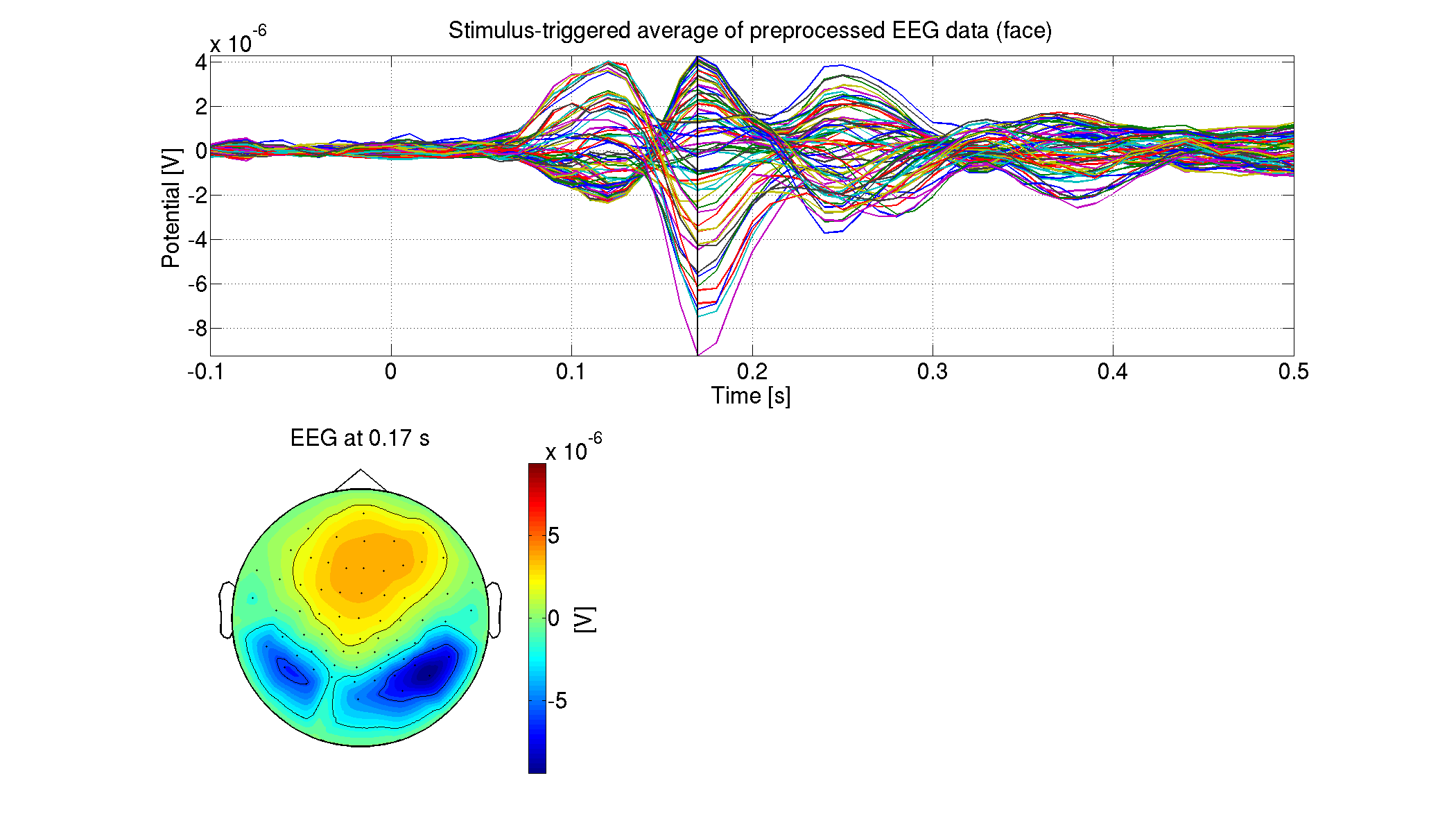
8.2.10. Showing preprocessed EEG data
For each condition, we show the processed EEG data averaged across the trials (vb_plot_sensor_2d.m).
>> show_preprocessed_eeg(p)
The following figure will be saved.
- $tutorial_dir/result/figure/show_preprocessed_eeg/sub-01/Face.png
8.3. Estimating source current from EEG data
We estimate source currents from the preprocessed EEG data.
8.3.1. Preparing leadfield
First, we construct a 3-shell (cerebrospinal fluid, skull, and scalp) head conductivity model for EEG source imaging (User manual, vb_job_head_3shell.m). Then, we make the leadfield matrix based on the head conductivity model (User manual, vb_job_leadfield.m).
>> prepare_leadfield_eeg(p)
The following files will be saved.
- $tutorial_dir/result/sub-01/eeg/leadfield/Subject.head.mat (3-shell head conductivity model)
- $tutorial_dir/result/sub-01/eeg/leadfield/Subject.basis.mat (Leadfield matrix)
8.3.2. Estimating source currents
First, we estimate the current variance by integrating the fMRI activity and the EEG data (User manual, vb_job_vb.m). Then, we estimate source currents using the current variance (User manual, vb_job_current.m).
>> estimate_source_current_eeg(p)
The following files will be saved.
- $tutorial_dir/result/sub-01/eeg/current/ctcAll.bayes.mat (Current variance)
- $tutorial_dir/result/sub-01/eeg/current/ctcAll.curr.mat (Source current)
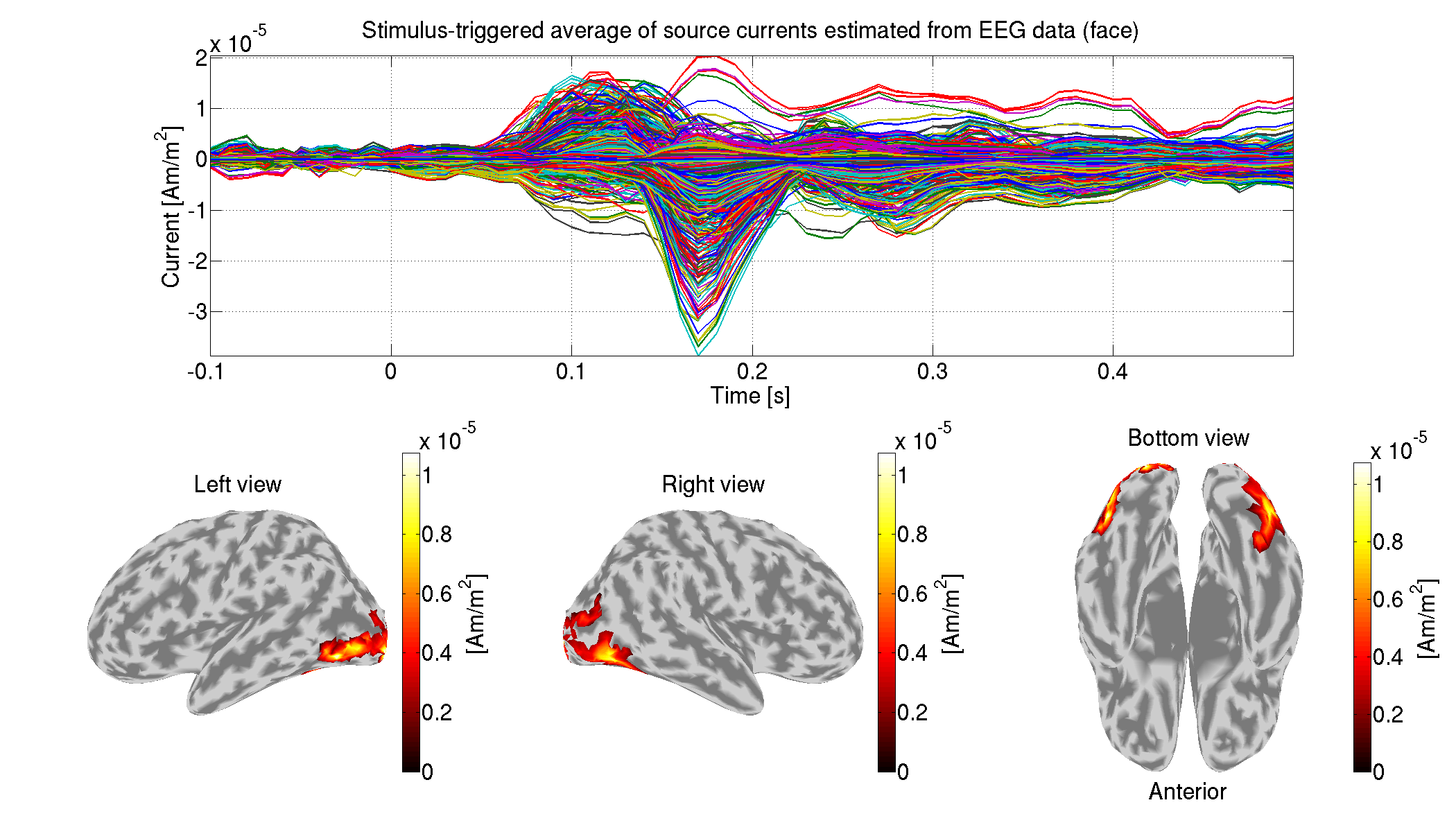
8.3.3. Showing estimated source currents
For each condition, we show the estimated source currents averaged across the trials (vb_plot_cortex.m).
>> show_source_current_eeg(p)
The following figure will be saved.
- $tutorial_dir/result/figure/show_source_current_eeg/sub-01/Face.png
8.4 Estimating source currents from both MEG and EEG data
Using VBMEG, we can estimate source currents from both MEG and EEG data.
8.4.1 Matching trials between MEG and EEG
We match the trials between the MEG and EEG data so that identical trials remain.
>> match_trial_meeg(p)
The following files will be saved.
- $tutorial_dir/result/sub-01/meg/trial/mtcAll.info.mat
- $tutorial_dir/result/sub-01/eeg/trial/mctcAll.info.mat
8.4.2. Estimating source currents
First, we estimate the current variance by integrating the fMRI activity, the MEG, and the EEG data (User manual, vb_job_vb.m). Then, we estimate source currents using the current variance (User manual, vb_job_current.m).
>> estimate_source_current_meeg(p)
The following files will be saved.
- $tutorial_dir/result/sub-01/meeg/current/mtcAll.bayes.mat (Current variance)
- $tutorial_dir/result/sub-01/meeg/current/mtcAll.curr.mat (Source current)
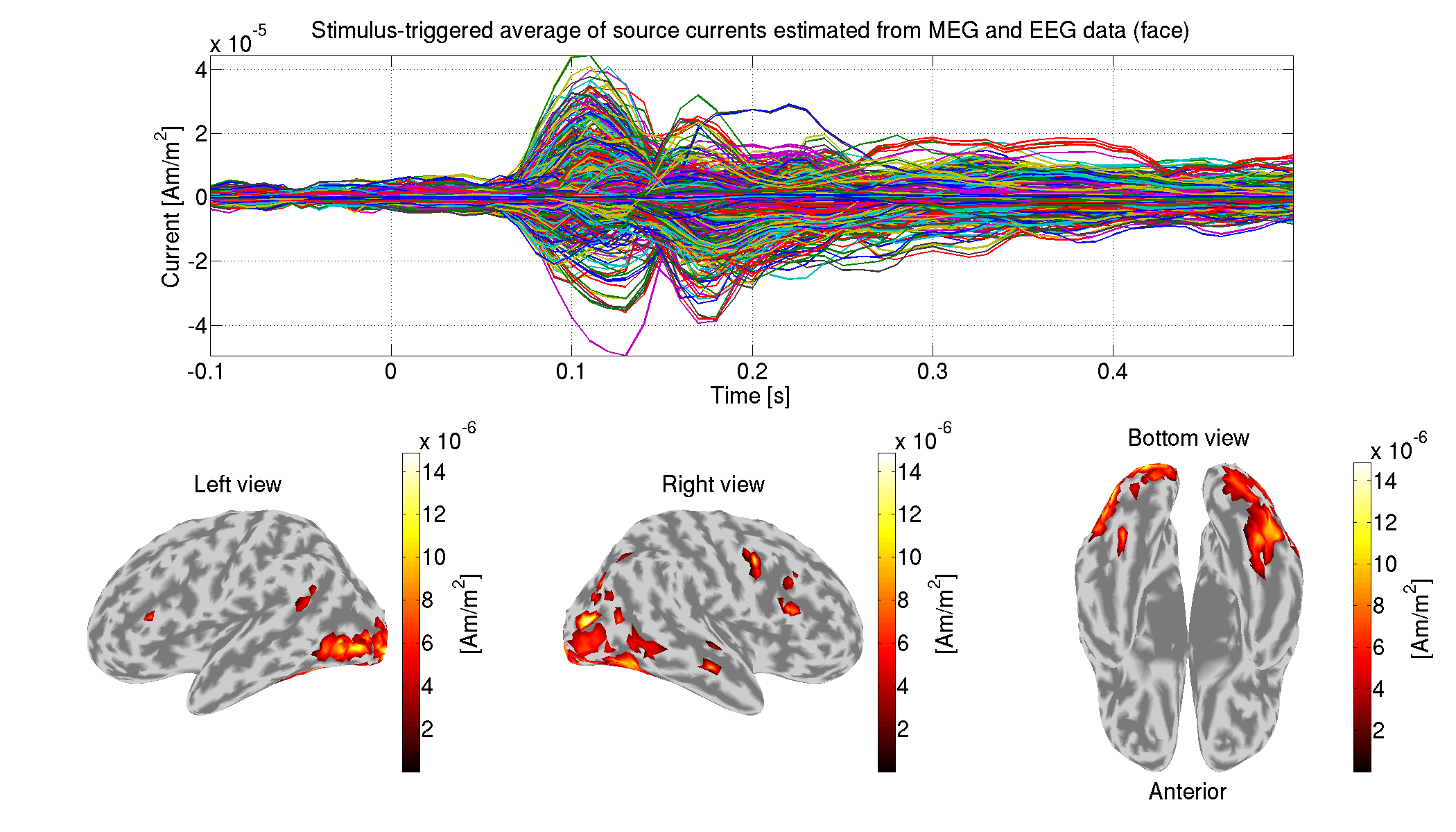
8.4.3. Showing estimated source currents
For each condition, we show the estimated source currents averaged across the trials (vb_plot_cortex.m).
>> show_source_current_meeg(p)
The following figure will be saved.
- $tutorial_dir/result/figure/show_source_current_meeg/sub-01/Face.png
9. Connectome dynamics estimation
In this section, we estimate a whole-brain connectome dynamics from the source currents estimated from the MEG data (User manual).
9.1. Adding path to necessary directory and setting subject number
We add path to dynamics directory and set the subject number to 1.
>> addpath('dynamics')
>> sub_number = 1;
>> p = create_project(data_root, tutorial_root, sub_number);
9.2. dMRI processing
To obtain an anatomical connectivity, which is used as a constraint for modeling connectome dynamics, we analyze the dMRI using FSL and MRtrix (User manual). The required environment for this dMRI processing is described in this document. You need to modify p.process_host, which specifies the list of host names, for your environment.
If setting the environment is difficult, you can skip over "9.2. dMRI processing" to "9.3. Estimating connectome dynamics" by putting the following files in your directories.
- $tutorial_dir/result/sub-01/dmri/connectivity/connectivity.dmri.mat
- $tutorial_dir/result/sub-01/brain/Subject_dmri.area.mat
9.2.1. Extracting brain from T1 image
We extract the brain (delete non-brain tissues) from the T1 image.
>> extract_brain_from_T1(p)
The following files will be saved.
- $tutorial_dir/result/sub-01/dmri/struct/Subject.nii.gz
- $tutorial_dir/result/sub-01/dmri/struct/Subject_brain.nii.gz
- $tutorial_dir/result/sub-01/dmri/struct/Subject_brain_mask.nii.gz
9.2.2. Importing dMRI
We copy dMRI files.
>> import_dmri(p)
The following files will be saved.
- $tutorial_dir/result/sub-01/dmri/dmri/dmri.nii.gz
- $tutorial_dir/result/sub-01/dmri/dmri/dmri.bval
- $tutorial_dir/result/sub-01/dmri/dmri/dmri.bvec
9.2.3. Correcting motion in dMRI
We correct motion in the dMRI.
>> correct_motion_in_dmri(p)
The following files will be saved.
- $tutorial_dir/result/sub-01/dmri/dmri/dmri_m.nii.gz
- $tutorial_dir/result/sub-01/dmri/dmri/dmri_m.bval
- $tutorial_dir/result/sub-01/dmri/dmri/dmri_m.bvec
9.2.4. Extracting brains from dMRI
We extract the brain (delete non-brain tissues) from the dMRI.
>> extract_brain_from_dmri(p)
The following file will be saved.
- $tutorial_dir/result/sub-01/dmri/dmri/dmri_m_brain_mask.nii.gz
9.2.5. Creating Fractional Anisotropy (FA) images from dMRI
We create an FA image from the dMRI.
>> create_fa_from_dmri(p)
The following file will be saved.
- $tutorial_dir/result/sub-01/dmri/dmri/fa_coreg.nii.gz
9.2.6. Coregistering T1 and cortical surface models to FA images
We coregister the T1 image and the cortical surface model to the FA images.
>> coregister_images(p)
The generated files will be saved in
- $tutorial_dir/result/sub-01/dmri/transwarp_info.
9.2.7. Removing noise in FA image
We remove the ambient noise in the FA image using the brain mask extracted from the T1 image.
>> remove_noise_in_fa(p)
The following file will be saved.
- $tutorial_dir/result/sub-01/dmri/dmri/fa.nii.gz
9.2.8. Parceling cortical surfaces
To define the seed and target region of interests (ROIs) used for fiber tracking, we parcel the cortical surface model.
>> parcel_cortical_surface(p)
The following file will be saved.
- $tutorial_dir/result/sub-01/dmri/parcels/parcels.mat
9.2.9. Parceling FA images based on parceled cortical surfaces
Based on the parceled cortical surface, we parcel the FA volume image.
>> parcel_fa_volume(p)
The generated files will be saved in
- $tutorial_dir/result/sub-01/dmri/parcels.
9.2.10. Creating masks for fiber tracking
We create a white matter volume file for fiber tracking.
>> create_mask_for_fiber_tracking(p)
The following files will be saved.
- $tutorial_dir/result/sub-01/dmri/fibertrack/wm.nii.gz (White matter)
- $tutorial_dir/result/sub-01/dmri/fibertrack/parcel_wm.nii.gz (Area mask)
9.2.11. Calculating fiber orientation density functions (FODF)
We calculate the FODF from the dMRI.
>> calculate_fodf(p)
The following file will be saved.
- $tutorial_dir/result/sub-01/dmri/fibertrack/CSD6.mif
9.2.12. Executing fiber tracking
Based on the FODF, we execute fiber tracking.
>> fiber_tracking(p)
The following file will be saved.
- $tutorial_dir/result/sub-01/dmri/fibertrack/anat_matrix.mat
9.2.13. Calculating connectivities
From the result of the fiber tracking, we calculate a binary connectivity matrix. Furthermore, we calculate the time lags between the ROIs based on the fiber lengths.
>> calculate_connectivity(p)
The following file will be saved.
- $tutorial_dir/result/sub-01/dmri/connectivity/connectivity.dmri.mat
- $tutorial_dir/result/sub-01/brain/Subject_dmri.area.mat
In Subject_dmri.area.mat, the ROI information, which vertex belongs to which ROI, is included.
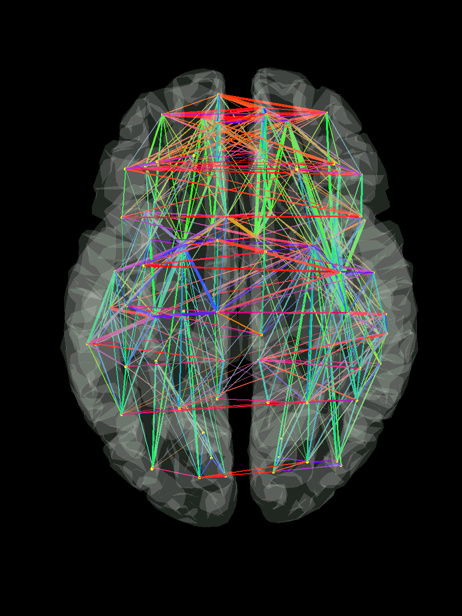
9.2.14. Showing connectivity
We show the estimated connectivity.
>> show_connectivity(p)
The following figure will be saved.
- $tutorial_dir/result/figure/show_connectivity/sub-01/brain.png
9.3. Estimating connectome dynamics
From the source currents estimated from the MEG data and the connectivity matrix, we estimate a linear dynamics model (Connectome dynamics estimation).
9.3.1. Calculating ROI current
We estimate a linear dynamics model between the ROIs defined in the dMRI processing. Therefore, we calculate the ROI current by averaging the source currents within each ROI.
>> calculate_roi_current(p)
The following file will be saved.
- $tutorial_dir/result/sub-01/dynamics/roi_current.mat
9.3.2. Estimating dynamics model
From the ROI current, we estimate a linear dynamics model using the L2-regularized least squares method, and in this model only the anatomically connected pairs of the ROIs have connectivity coefficients (Connectome dynamics estimation).
>> estimate_dynamics_model(p)
The following file will be saved.
- $tutorial_dir/result/sub-01/dynamics/dynamics_model.lcd.mat
9.4. Creating movie
We create the movie displaying the signal flows between the ROIs (User manual).
9.4.1. Preparing input for creating movie
To create the movie, we need
- The ROI current,
- The dynamics model,
- The place of the ROIs,
- Time information.
We gather these from separate files.
>> prepare_input_for_movie(p)
The following file will be saved.
- $tutorial_dir/result/sub-01/dynamics/input_for_movie.mat
9.4.2. Executing fiber tracking
If you skipped "9.2. dMRI processing", you also need to skip this "9.4.2. Executing fiber tracking" by putting Vmni_connect.mat in $tutorial_dir/result/sub-01/dynamics/.
For the important pairs of the ROIs, we execute the fiber tracking again to obtain the shapes of the fibers.
>> fiber_tracking_for_movie(p)
The following file will be saved.
9.4.3. Creating movie
We create the movie displaying the signal flows.
>> create_movie(p)
The following movie will be saved.
Congratulations! You have successfully achieved the goal of this tutorial.