VBMEG users manual
Contents
- Contents
- 1.Introduction
- 2.Process overview
- 3.Project
- 4.Brain modeling
- 5.fMRI import
- 6.M/EEG data processing
- 7.Source imaging
- 8.Connectome dynamics
- A-1.VBMEG APIs
- A-2.Tips
- A-3.Troubleshooting
- A-4.References
- A-5.Acknowledgement
1.Introduction
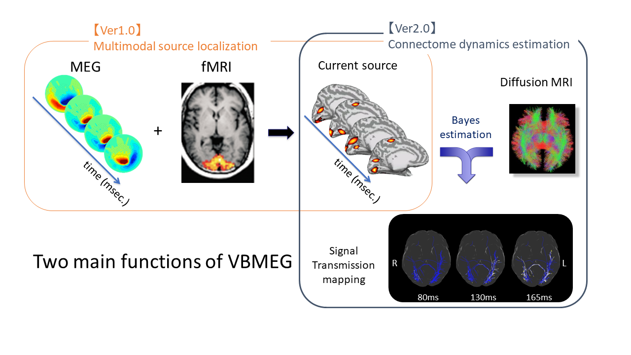
VBMEG (Variational Bayesian Multimodal EncephaloGraphy) is a Matlab toolbox for MEG/EEG current source imaging and connectome dynamics estimation. As its name stands, VBMEG is originally intended to obtain accurate source image in individual brain basis by integrating currently available brain imaging modalities (MEG,EEG,fMRI,T1-MRI,dMRI).
VBMEG is based on the hierachical Bayesian model (application of automatic relevance determination developed by D.Mackay 1992) and uses fMRI activity map as prior knowledge for source estimation and yields accurate source localization (Sato et al.2004). Even without fMRI, VBMEG works and provides sparse current source imaging which is rather accurate for event-related brain activities.
The first version has been made available as open source software since 2011 and used in several research projects in other groups (Toda et al.2011, Yoshimura et al. 2012, Callan et al. 2016, Yanagisawa et al. 2016, Yoshimura et al. 2017). This new version provides additional functions including connectome dynamics identification method (Fukushima et al. 2015) connectome dynamics visualization method, and MEG+EEG simultaneous source imaging method.
What you can do with VBMEG
Using VBMEG one can:
- Brain modeling
- Cortical model
- Head model(1shell:MEG, 3shell:EEG)
- M/EEG data processing (Yokogawa, Biosemi, BrainAmp).
- fMRI data import from SPM8(SPM:statistical parametric mapping).
- Source Imaging
- Calculate M/EEG forward model (leadfield).
- Estimate M/EEG inverse filter.
- Estimate cortical current.
- Connectome dynamics
- Diffusion MRI (dMRI) processing
- Connectome dynamics estimation
- Create dynamics movie
"Our full-set pipeline requires MEG,EEG,fMRI,T1,dMRI and sensor positions (link) while our minimum-set pipeline only requires EEG (link). Required data depends on what you do with VBMEG."
Requirements
- Hardware
- Windows 7/10 or Linux(x86/x64), any other operating system is not supported.
- Software
- VBMEG is running on MATLAB environment (version 7.0 to 2014a).
- FreeSurfer4.2 or later is needed to create cortical surface model (gray matter/white matter boundary).
- MRtrix 0.2.1x and FSL 4.1 or later are needed for dMRI processing to obtain connectome.
- SPM8 is needed for fMRI data processing.
Supported data formats
- Structural MRI data (NIfTI/ANALYZE).
- Cortical surface model (FreeSurfer).
- MEG data (Yokogawa/Neruomag)
- EEG data (Biosemi/BrainAmp).
- Sensor position data (Fastscan).
- fMRI data (SPM8).
- Head model (SPM8 and FreeSurfer;).
- Tractography (connectome) (output of MRtrix)
2.Process overview
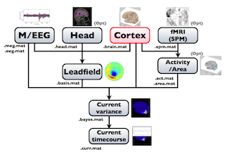
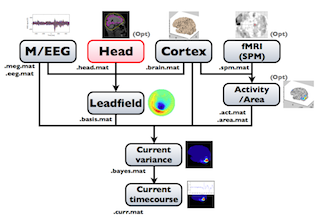
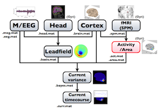
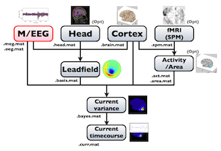
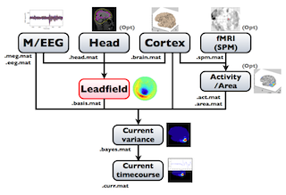
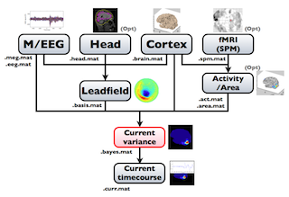
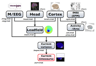
The following figure is a diagram of VBMEG processes for source imaging. The overview of connectome dynamics is described in the section "Connectome Dynamics".
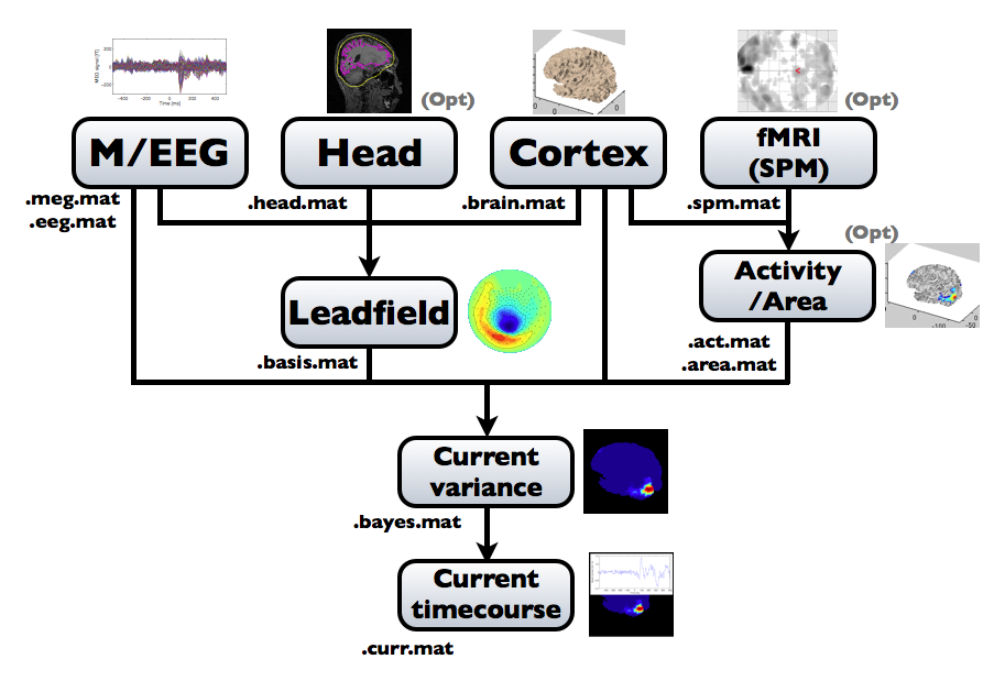
Brain modeling("Cortex", "Head"), M/EEG data processing("M/EEG"), fMRI activities import("Activity/Area") and source imaging("Leadfield", "Current variance", and "Current timecourse") steps can be performed on GUI.
VBMEG file type
The following files are created by VBMEG:
- Cortical surface model file (.brain.mat) a polygon model of gray/white matter boundary, inflated model for displaying purposes, and information related to the model.
- Cortical activity file (.act.mat) consists of sets of some kind of activities (e.g., SPM t-value, cortical current at a time point) on the cortical surface model.
- Cortical area file (.area.mat) consists of sets of vertex indices representing a particular brain region (which can be the whole cortex) of the cortical surface model. For each vertex set, a string key is assigned, which is used to get the vertex set.
- M/EEG file (.meg.mat/.eeg.mat) has time-courses of M/EEG signals and extra channels.
- Head model file (.head.mat) has information about the structure of the subject's head. It is used to calculate the forward model by a numerical method (BEM).
- Leadfield file (.basis.mat) has leadfield matrix, which depends on the cortical surface model, head model, and M/EEG sensor position information included in the M/EEG-MAT file.
- Current variance file (.bayes.mat) has estimated current variance values and other model parameters of the hierarchical model of the M/EEG inverse problem.
- Cortical current file (.curr.mat) has estimated cortical currents.
3.Project
What is a project?
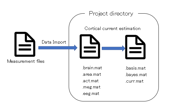
Project is a framework for managing measurement data, analysis data, and analysis parameters. Whatever you do in VBMEG, you do that in the context of the project.
- Project
- Project is just a directory, and the directory is called "project root" or "proj_root".
- Data Import
- An operation to add measurement data(MRI,fMRI,M/EEG data) to project.
Set path
Execute the following commands in MATLAB in order to run the software:
> addpath(fullpath_to_vbmeg);
> vbmeg;
--- Find VBMEG program directory
VBMEG program directory: /home/cbi/rhayashi/vbmeg
--- Set program directories to MATLAB path
--- Create global variable 'vbmeg_inst'
Here, the variable fullpath_to_vbmeg indicates the path of the top directory of the VBMEG software (“vbmeg”). If only the relative path is given, part of the GUI might not work properly. While the path settings will be preserved until MATLAB is closed, the command vbmeg has to be executed every time the memory is cleared, since this command defines a global variable ("vbmeg_inst").
Project manager startup
The project manager manages the execution of the various VBMEG GUIs and the parameters involved in each operation. It can be called after executing the vbmeg command by entering the following:
> project_mgr
The project manager GUI is shown.
Screen description
The project manager saves the time and parameters at which the analysis was executed.
In addition, it launches GUI for viewing / editing data created by analysis, and outputs M-Script which can be executed in batch.
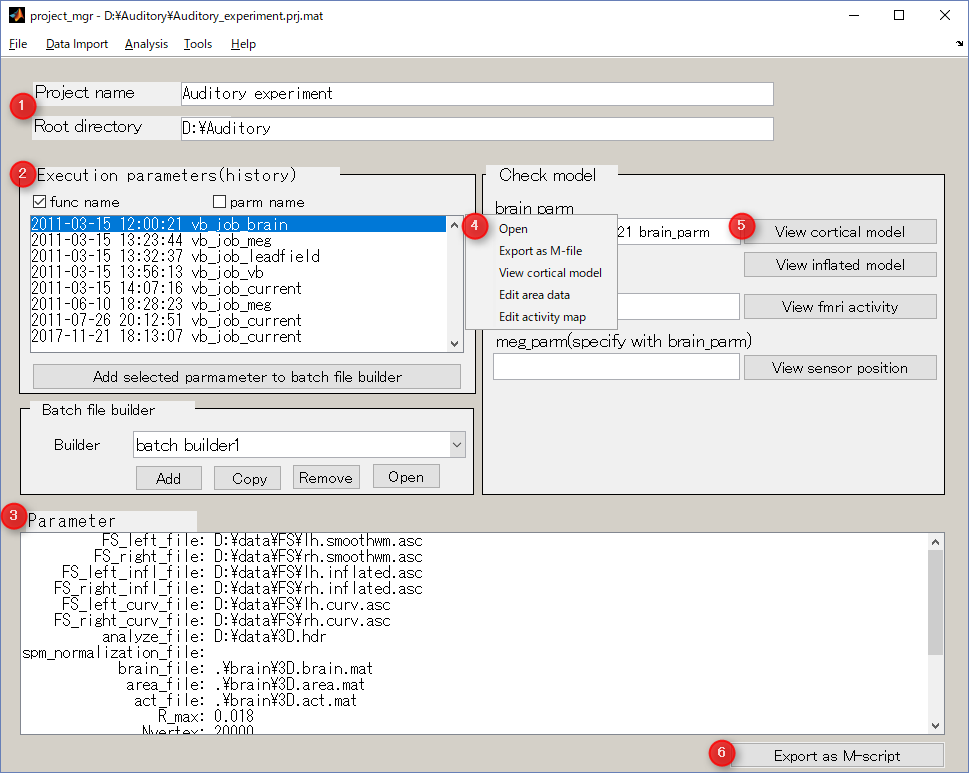
- Project name and project directory
Display information on the project.
- Execution parameters(history)
History of analysis date, time and parameters.
- Parameter
Display details of the parameter selected item in 2:Execution parameter.
- Context menu
- "Open"
- Open GUI using this parameter.
- "Export as M-file"
- Save selected parameter as a executable M-file.
- Others
- Open the data viewer/editor according to selected parameter.
- Check model button
- "View cortical model"
- Display cortical model.
- "View inflated model"
- Display inflated cortical model.
- "View fMRI activity"
- Display imported fMRI activity.
- "View sensor position"
- Display cortical model and sensors.
- Export as M-script
Saves selected parameter as an executable M-file.
Create new project
Creating a new project file
- From the project manager menu select [File]->[New project], then "Create new project" GUI will pop up.
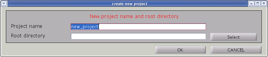
- Input “Project name” and ”Root directory”, the directory in which the project should be saved. Press "OK" button.
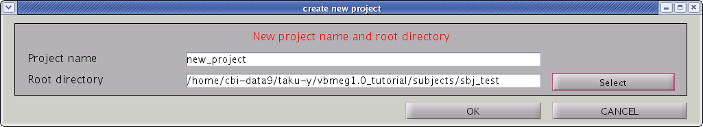
- Confirmation dialog will pop up. Press "OK" button.
Specifying an existing project file
- From the project manager menu select [File]->[Load project], then the file select dialog will pop up.
- Specify the project file.
- "Project name" and "Root directory" will be appeared in their respective line of the project manager dialog.
4.Brain modeling
VBMEG can utilize cortex polygon models created with FreeSurfer. It automatically extracts cortical surface models from the MRI data. This section explains how to prepare MRI file, execute FreeSurfer, and import cortical model. From version 2.0, VBMEG adopts the MNI-aligned individual brain model. Vertex points of all individual brain models are aligned with MNI coordinate of the standard brain (ISBM152). This model makes group-level current source analysis much easier.
MR image preprocessing
DICOM to NIfTI conversion
MRI data are required to create subject's cortical surface model which is often provided with DICOM format. However, since VBMEG supports NIfTI(Analyze) format, DICOM files can be converted to NIfTI file(.nii) with VBMEG function convert_dicom_nifti.
- Function name
- convert_dicom_nifti
- Description
- This function converts DICOM files to NIfTI(.nii) format. The origin is set to the center of the image by this operation. Verify that NIfTI file is created for using this function. Running this function, NIfTI file(.nii) with prefix 'RAS_' is created.
- Syntax
- convert_dicom_nifti(dicom_file, output_dir);
- Parameters
-
- dicom_file
- a filename of an arbitrary DICOM file consisting MRI. (e.g.1.3.12.2.1107.5.2.32.35283.2013103111331835928852729.dcm)
- output_dir
- output directorty for NIfTI file.
- Remarks
- If no parameters are specified, file selection dialog opens. Selecting one of DICOM files and pressing the OK button, NIfTI file will be created in the same directory as the DICOM file.
Bias correction
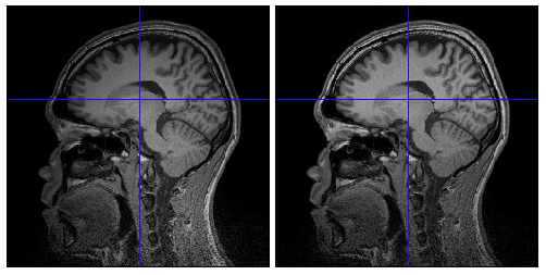
Because of inhomogeneous magnetic field, MR images are sometimes contaminated by low frequency variation of signal values, which adversely affects on extraction of cortical surface from the images. VBMEG function vb_bias_correction_by_spm can be used to correct signal values of MR images. Before executing this function, you need to set MATLAB path to SPM8 directory. The following figures are MR images before and after bias correction.
- Function name
- vb_bias_correction_by_spm.
- Description
- Bias correction is applied to specified MRI file. Running this function, bias corrected MRI file with prefix 'm_' is created in the same directory as the original file.
- Syntax
- vb_bias_correction_by_spm(mri_file);
- Parameters
- mri_file : NIfTI file(.nii)
- Remarks
- SPM8 should be added to your MATLAB(e.g. addpath(genpath('SPM8path'))
Cortical surface model
Cortical model creation
VBMEG has a function to call FreeSurfer to create a cortical model.
- Function name
- vb_freesurfer_run
- Description
- This function creates FreeSurfer command and gives it to FreeSurfer.
- Syntax
- vb_freesurfer_run(mri_file, fs_root_dir, subj_id);
- Parameters
-
- mri_file
- MRI file(.nii) which is created using convert_dicom_nifti function.
- fs_root_dir
- Root directory of FreeSufer
- subj_id
- Cortical model file are put to the fs_root_dir/subj_id directory.
- Setup
- Please write FreeSurfer program path in a $VBMEG/vbmegrc.($VBMEG :VBMEG program directory)
> edit vbmegrc
# vbmeg resource file for bash shell.
# for FreeSurfer
FREESURFER_HOME=/home/software/freesurferv4.5.0 - Run vb_freesurfer_run with the arguments.
- Example
> vb_freesurfer_run('/home/mri/Subject.nii', '/home/FS_ROOT_DIR', 'SUBJ_ID');
creates /home/FS_ROOT_DIR/SUBJ_ID from the /home/mri/Subject.nii It will take about 12-24 hours on a Linux PC.
recon-all command
To execute the FreeSurfer command directly, please refer to the following.
mri_convert sbj_test.nii 001.mgz
'001' denotes that it is the 'first' MR image. FreeSurfer can construct the cortical surface model using two or more MR images (of the same subject) by averaging them to increase S/N ratio of the MR image from which the cortical surface model is extracted. In that case, subsequent MGZ filename should be '002', '003', etc.
To create the FreeSurfer's subject directory, you can use mksubjdirs command as follows:
mksubjdirs $SUBJECTS_DIR/sbj_test
'sbj_test' is ID of the subject. All MGZ files have to be put in the $SUBJECTS_DIR/[sbj_id]/mri/orig/ directory as shown below:
cp 001.mgz (002.mgz 003.mgz ... if any) $SUBJECTS_DIR/sbj_test/mri/orig
The recon-all command processes MR image(s): (GM/WM boundary extraction, coregistration to the template, etc.) as in the following example:
recon-all -all -subjid sbj_test
After completion, surface files of the polygon model are saved in binary format. For VBMEG, the FreeSurfer data has to be saved in ASCII format. This can be done using the mris_convert command included with FreeSurfer. Executing the following commands in an Unix shell generates the files necessary for import of the cortical surface model into VBMEG:
cd [freesurfer_sbjdir]/sbj_test/surf/
mris_convert [lh/rh].smoothwm ../bem/[lh/rh].smoothwm.asc
mris_convert [lh/rh].inflated ../bem/[lh/rh].inflated.asc
mris_convert -c curv [lh/rh].smoothwm ../bem/[lh/rh].curv.asc
mris_convert [lh/rh].sphere.reg ../bem/[lh/rh].sphere.reg.asc
Cortical model files
Freesufer creates cortical model files as below.
| cortical surface | bem/[lh|rh].smoothwm.asc |
|---|---|
| inflated surface | bem/[lh|rh].inflated.asc |
| curvature | bem/[lh|rh].curv.asc |
| spherical registration info | bem/[lh|rh].sphere.reg.asc |
| inner skull surface(CSF) | bem/inner_skull_surface.asc |
| head skin surface | bem/outer_skin_surface.asc |
| cortex label | label/[lh|rh].cortex.label |
Import cortical model
- VBMEG function: vb_job_brain
- From the project manager menu select [Data Import]->[Import cortical model]. "Import cortical model" GUI will pop up.
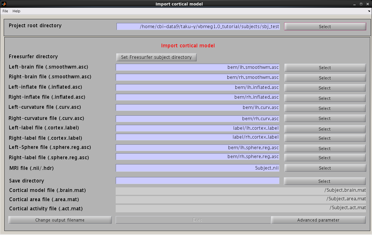
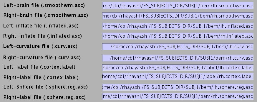
- Press the "Set FreeSurfer subject directory" button, dialog appears. In the appearing dialog, specify FreeSurfer subject directory and press the "Apply" button.
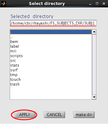
All the FreeSurfer files are automatically set.
- Specify NIfTI file of subject's MRI from which the cortical surface model was extracted FreeSurfer).

- Specify the directory to which created files are saved.

- Filenames are automatically set using MRI filename.

- Press “Exec” button to start import of the cortical model.
After processing, three files will be created: the cortical surface model file (.brain.mat), cortical activity file (.act.mat) and cortical area file (.area.mat). The following figure will be shown. Check if the cortical surface model (yellow dot) is aligned with the gray/white matter boundary in MR image.
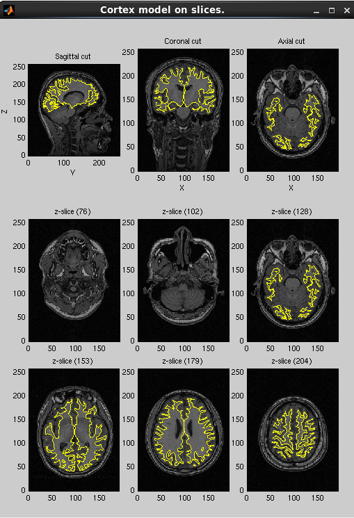
In addition, VBMEG creates three more files: _brodmann.area.mat, _aal.area.mat, and _atlas.act.mat, which include anatomical label data on the cortical surface model.
Head model
You can use a spherical model to create the M/EEG forward model (leadfield). The spherical model is specified by the origin of the sphere and its radius. The MEG forward model with a spherical model is analytically calculated by the Sarvas equation which is not dependent on the radius of the sphere, while radii of spheres are also required for three-layers EEG forward model.
To obtain a more accurate forward model, VBMEG can create a cranial model from the subject's MRI. The required files for this calculation are:
- volumetric image of gray matter(c1*.nii). (see What is gray matter file and SPM normalization file?)
- inner skull and outer skin surface files, created by FreeSurfer(see Cortical model files)
Import head model
- VBMEG function: vb_job_head_3shell
You can make a realistic head model to improve accuracy of the leadfield calculation by following the steps below:
- Select [Data Import]->[Import head model] from the project manager menu. "Create head model" GUI will pop up.
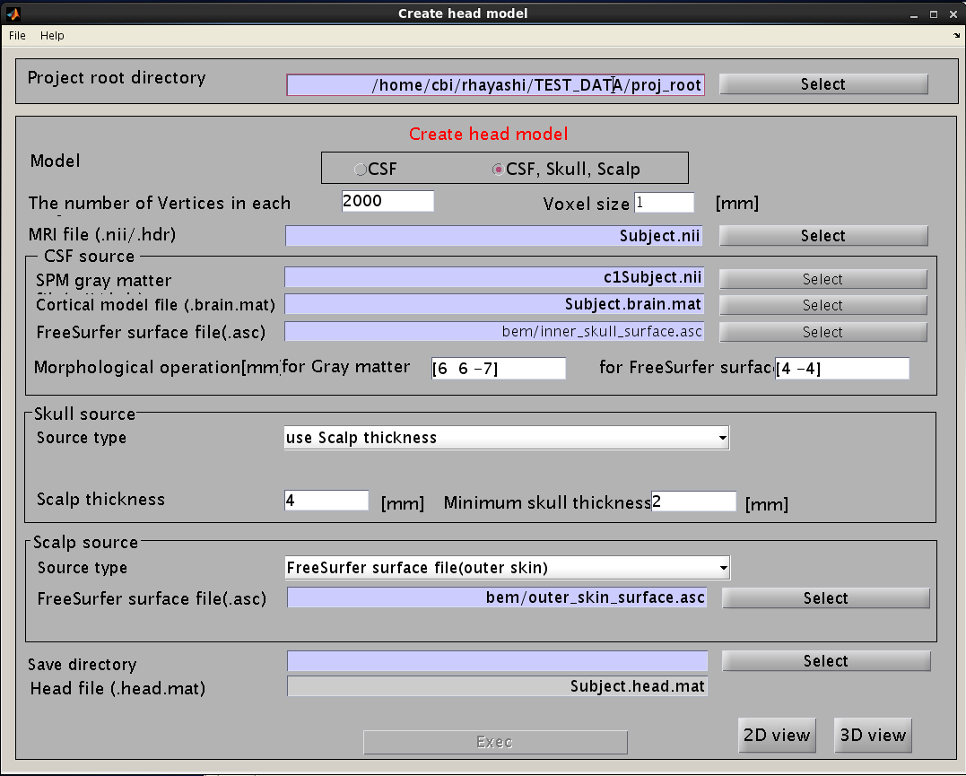
- Specify files and parameters.
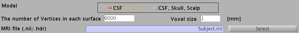
- Specify head model type. For MEG check "CSF", making a head model consisting of single layer (celebro-spinal fluid; CSF). Then the number of vertices of the CSF layer is automatically set (6,000 by default). The Analyze/NIfTI image is also required.
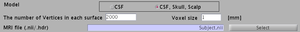
- For EEG, check "CSF, Skull, Skalp", which will make a head model consisting of three layers (CSF, Skull, Scalp). The number of vertices for each of the three layers is 2,000.
- Specify files and parameters for creating the CSF surface. The required files are the SPM8 gray matter file (c1*.hdr), VBMEG cortical surface model file, and FreeSurfer inner skull surface file (see section "Head model" of "Preparation of files required for VBMEG").
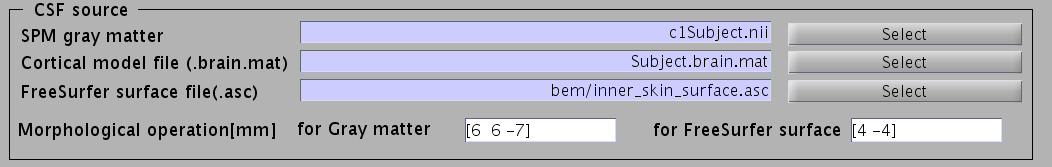
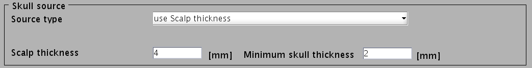
- Specify parameters for creating the skull surface. You can use the default parameters.
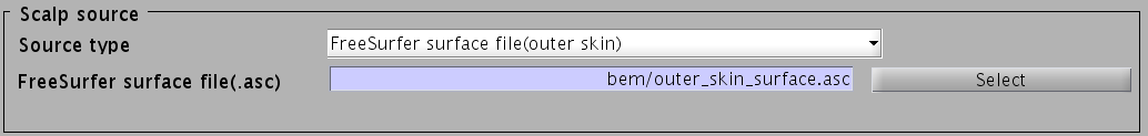
- Specify files and parameters for creating the scalp surface. The required files are FreeSurfer outer skin surface file (see section "Head model" of "Preparation of files required for VBMEG").
- Specify the directory to which the head model file is saved.

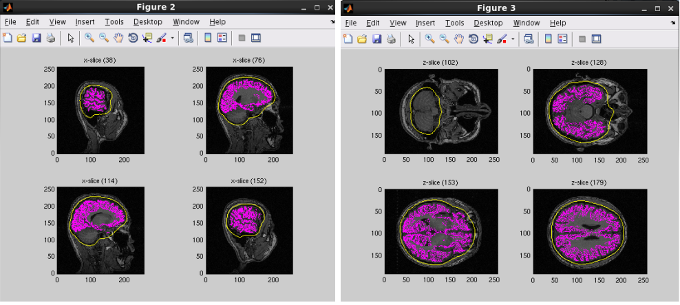
- Press "Exec" button to start making the head model.
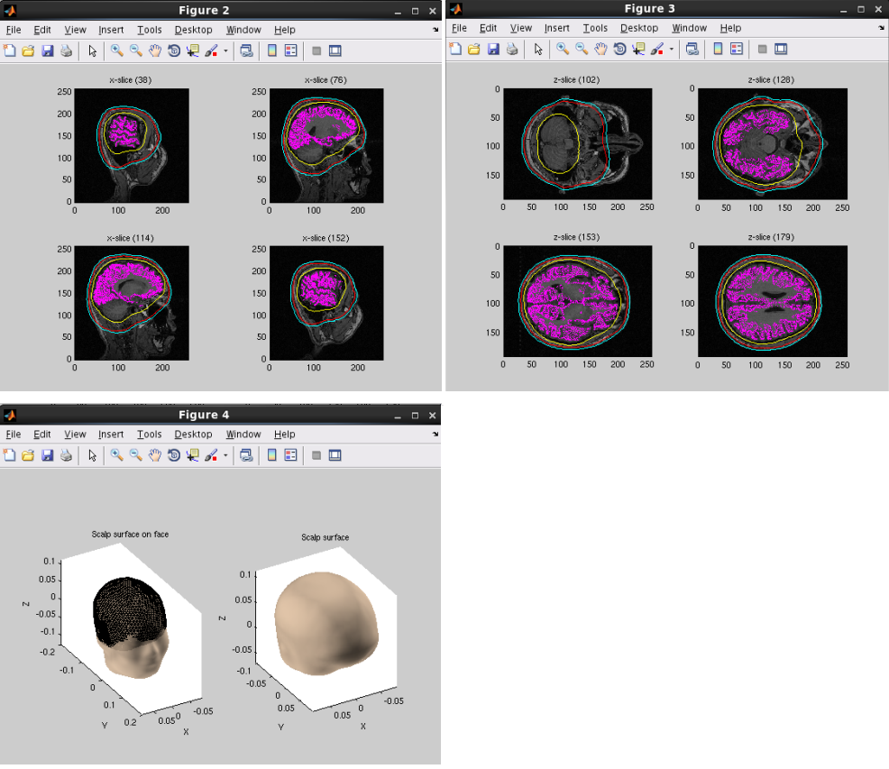
A head model file will be created and below figures will be appeared. In this example there is a CSF single layer (yellow line) model for MEG. Check if the CSF surface correctly aligned with the MR image.
Specifying a three layer model for EEG gives the following figures, consisting of CSF (yellow), skull (red), and scalp (light blue) surfaces. In the last figure, the scalp surface is superimposed on the face model.
5.fMRI import
Source current estimation from M/EEG measurement is an ill-posed problem. If you have fMRI information, VBMEG uses it as prior knowledge for source estimation and yields more accurate source localization.
SPM8 generated t-values can be used to determine the relative amplitude of the prior current variance in the hierarchical Bayesian estimation.
VBMEG assumes that fMRI analysis is performed on the standard brain. To import it, you need to create a SPM normalization file(_sn.mat).
Import fMRI data
- VBMEG function: vb_job_fmri
SPM-Voxel file (SPM.mat) can be imported by following the steps below:
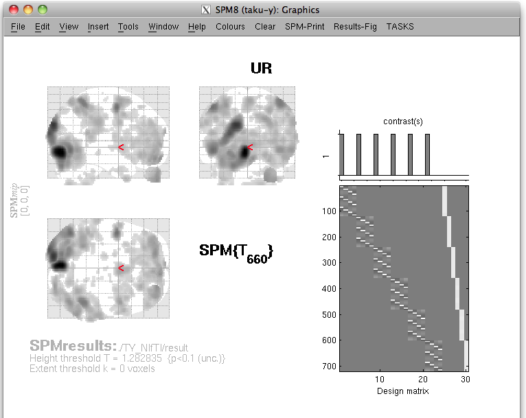
- Select [Data Import]->[Import SPM data] from the project manager menu. "Import SPM voxel data" GUI will pop up.
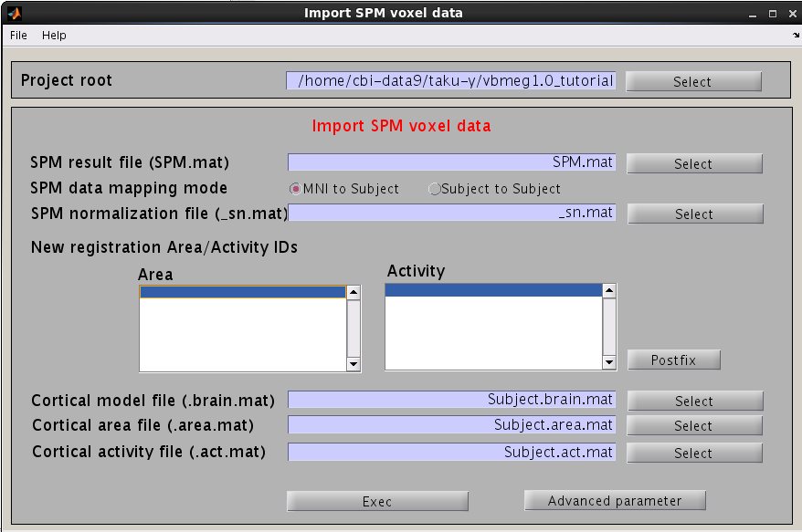
- Specify SPM.mat file which is created by SPM8.

- New registration Area/Activity IDs are shown.
_T : T-value
_PS : Percent signal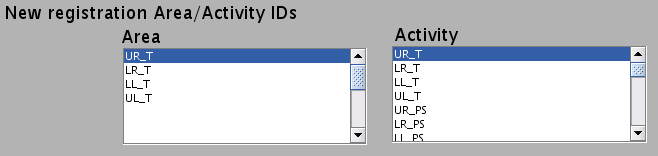
- New registration Area/Activity IDs are shown.
- Specify the cortical surface model file (.brain.mat), onto which voxels are projected.

- Specify the cortical activity file and cortical area file. The activity map and cortical area are stored in these files with specified IDs.

- Press “Exec” button to start the data import.
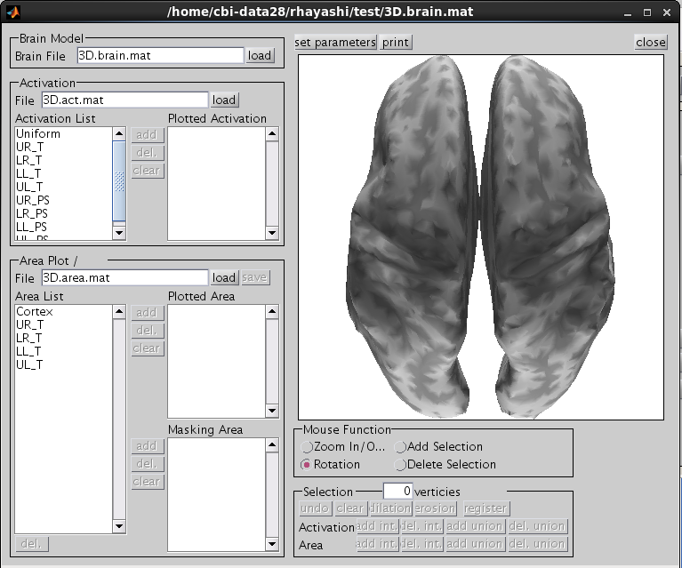
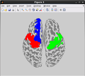
The t-values provided by the SPM-Voxel file are mapped onto the cortex vertices and registered in the cortical activity file with the identifier you have specified. Additionally, voxels with a t-value exceeding the threshold will be registered as an individual area of the cortex and saved in the cortical area file. The following figure appears.
Choose one of the activity and press the add button.
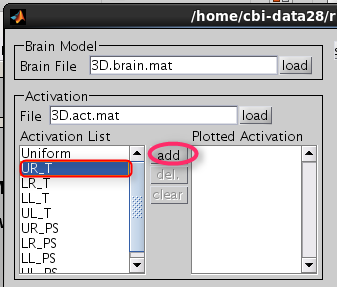
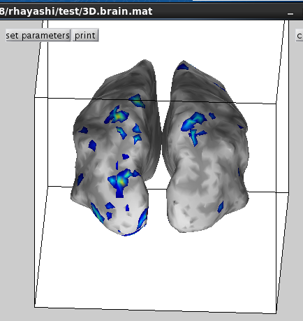
Then selected activity will be plotted on the cortical model.
6.M/EEG data processing
VBMEG provides GUI for some basic process of MEG/EEG data preprocessing, including data import, digital filtering and trial extraction but does not provide GUI for advanced process such as artifact rejection/removal. One convenient way to perform the whole preprocess pipeline is to use a script file. You can refer to our full connectome-dynamics estimation tutorial. The other convenient way is to use other sophisticated toolbox such as EEGLab and BrainStorm and then convert results to VBMEG format. Here we explain GUI operation for data importing and checking.
Import MEG data
- VBMEG function: vb_job_meg
VBMEG can import MEG data measured by a Yokogawa system (MegLaboratory; .raw, .ave, .con). The MEG sensor position should be transformed into VBMEG coordinate system(RAS, origin at the center of MRI volume, m). The coregistration methods supported by VBMEG are the standard method offered by MegLabotory (determination of the marker location by means of MRI) and the method developed by Shimadzu and ATR (three dimensional matching of the face; Kajihara et al., 2004). To import MEG data, follow the below steps:
- Select [Data Import]->[Import MEG data]->[Yokogawa] from the project manager menu. "Import YOKOGAWA MEG data" GUI will pop up.
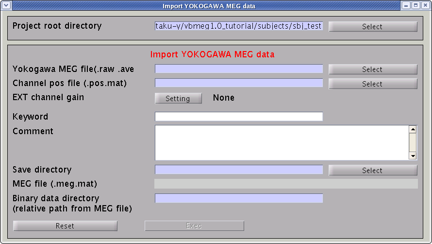
- Specify the required MEG data files.
- Specify Yokogawa MEG file (.raw, .ave, .con).

- Specify positioning file (.pos.mat). This is used to transform sensor coordinate values.

- Specify the directory to which created file will be saved.

- The MEG-MAT file name is automatically set. In addition, the directory, in which the MEG time course is saved, is also created.

- Press “Exec” button to start the import.
The data, now formatted for VBMEG, are saved in a MEG-MAT file.
Import EEG data
- VBMEG function: vb_job_meg
Data obtained by a Biosemi EEG system (.bdf) can also be imported. Screening of the individual session and trial data for artifacts is recommended before the import, but can also be conducted after the import into VBMEG. The EEG sensor position has to be transformed into SPM-Analyze (RAS, origin at the center of MRI volume) coordinate system before import. The coregistration method supported by VBMEG is the one developed by Shimadzu and ATR (three dimensional matching of the face; Kazihara et al., 2004). EEG data can be imported by following the steps below:
- Select [Data Import]->[Import EEG data]->[Biosemi] from the project manager menu. "Import Biosemi EEG data" GUI will pop up.
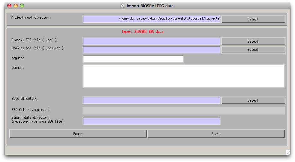
- Specify the required EEG data files.
- Press “Exec” button to start the import, then the channel lists, included in the BDF file and the POS-MAT file, are shown. The order of channels does not matter, but you should check if all the EEG channels (on the scalp) in the BDF file are included in the POS-MAT file. Some extra channels (EOG, EMG, trigger recording) can be included in the BDF file, so the lengths of the lists can also be different. Pressing "Sort" button sorts the order of the display and does not affect import process.
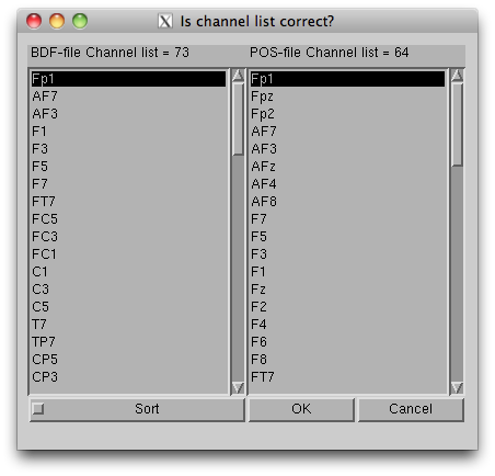
The data, now formatted for VBMEG, are saved in an EEG-MAT file (.eeg.mat).
Showing M/EEG data
To check signals of MEG data, you can use M/EEG viewer. Select [Tools]->[View MEG/EEG data] from the project manager menu. Then "View MEG/EEG data" dialog will pop up.
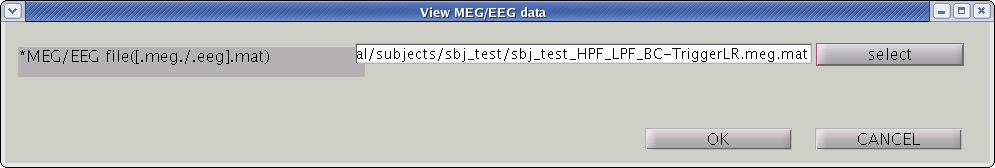
Select MEG-MAT file and press "OK" button. MEG/EEG viewer GUI will pop up.
Screen description
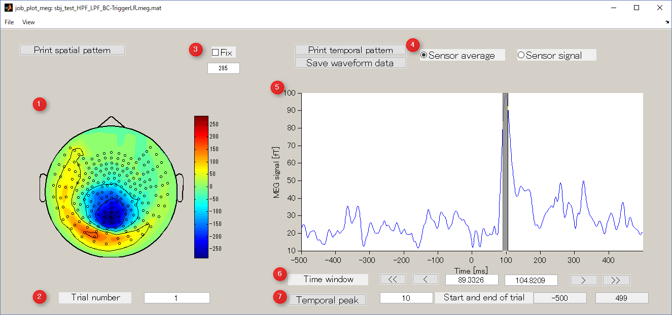
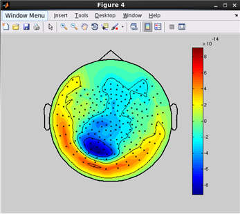
- Spatial map
Display spatial pattern of M/EEG data averaged over the selected time window.
- Trial number
Display M / EEG data of the specified trial number.
- Colorbar
It is used to specify the absolute value of the data to be displayed. Normally, when you select the time window, the value is automatically updated, but if you check Fix box, it will be fixed to the value specified in the editbox.
- Sensor average/Sensor signal
Waveform display mode.
- Sensor average
Root mean square of sensor data is displayed.
- Sensor signal
Raw sensor data is displayed.
- Sensor average
- Waveform of sensor data
Sensor average or sensor signal is displayed. You can select the time window for calculating the spatial map by dragging the left mouse on the graph.
- Time window
It is an interface that displays and specifies a time window for averaging sensor timeseries.
- Temporal peak button
This button is used to find the peak of timecourse.
Select arbitrary time window
you can select arbitrary time window, from which the spatial map is obtained, by dragging the cursor on the right panel.
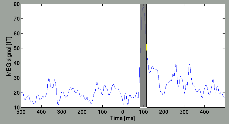
Then, the spatial map will be updated.
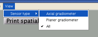
Select sensor type
The spatial map may be discontinuous due to the configuration of the direction in sensors of some MEG systems is arbitrary (as of MEG system in ATR). You can select axial sensors to be plotted from the menu of GUI.
Sensor selection method
When you right-click on the spacial map, the sensor selection method menu is displayed(Brush/Lasso/Rect).
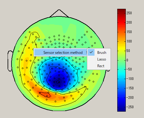
| Brush | Lasso | Rect |
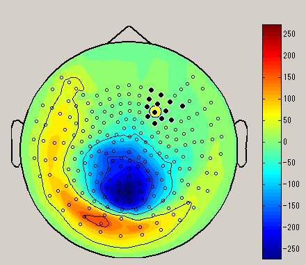 |
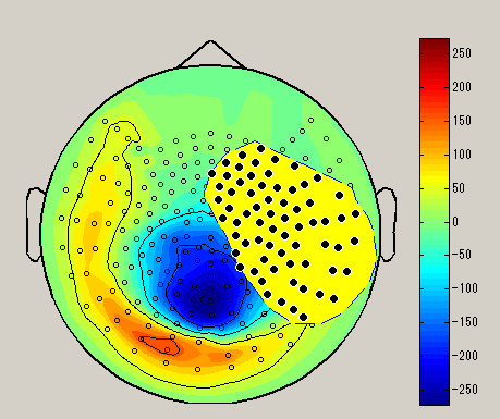 |
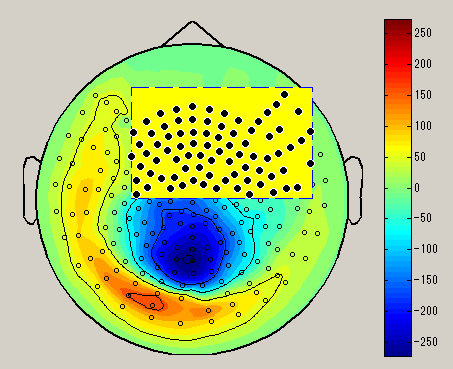 |
| Select sensor with a small circle | Select sensor with lasso | Select sensor with rectangle |
After choosing the sensor selection method, select the sensor by dragging left mouse on the spacial map. (Black circle : selected sensor), the data of the selected sensor will be displayed on the graph. To unselect, left click on outside the sensor.
7.Source imaging
The estimation of the current source with VBMEG is done in three steps: Leadfield calculation, current variance estimation and finally, current timecourse estimation.
Leadfield calculation
- VBMEG function: vb_job_leadfield
VBMEG implements the following leadfield matrix computation.
- MEG
- an individual brain model (boundary element method (BEM), spherical harmonic expansion)
- a spherical head model
- EEG
- an individual brain and three-shell head model (BEM)
- a spherical three-shell head model
- the standard brain and three-shell head model (BEM)
Here we explain how to obtain MEG leadfield matrix for an individual brain with BEM.
- Select [Analysis]->[Calculate leadfield] from the project manager menu. The "Leadfield calculation" GUI will pop up.
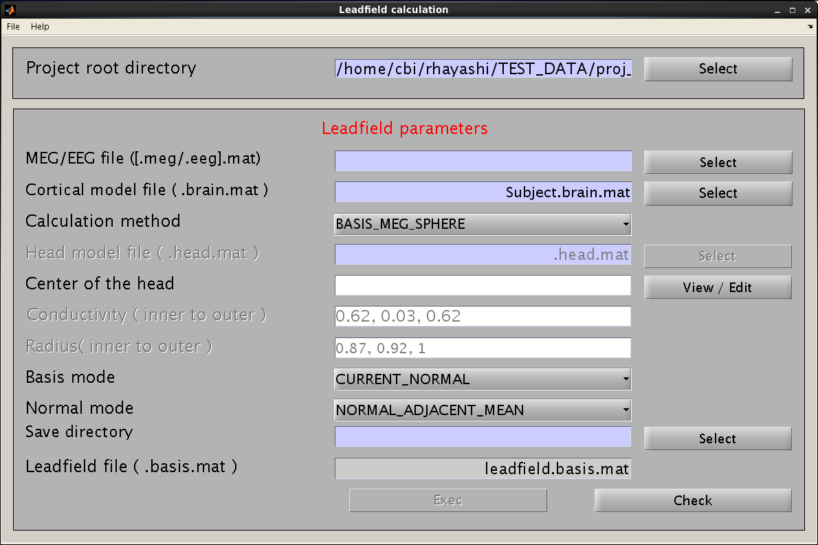
- Specify the required files and parameters.
- Specify the M/EEG-MAT file and cortical model file. You do not need to specify the cortical area file (the field is not necessary and will be removed in a future version).

- Specify the method for leadfield calculation. "BASIS_MEG_BEM" is the option to use BEM for calculation of the leadfield.

- The head model file must be specified for BEM.

- Do not modify parameters here. These parameters are used for advanced users.

- Specify the directory to which the leadfield file is saved. The filename is automatically set using the MEG-MAT filename.

- Specify the M/EEG-MAT file and cortical model file. You do not need to specify the cortical area file (the field is not necessary and will be removed in a future version).
- Press “Exec" button to start the leadfield calculation.
- The result is saved in the leadfield file (.basis.mat).
The leadfield at M/EEG sensors are calculated for every vertex of the cortical surface model.
Current variance estimation
- VBMEG function: vb_job_vb
The hierarchical Bayesian method estimates variance of the current from the MEG data. Once the current variance is obtained, we can calculate the linear inverse filter, which will yield the current estimation when multiplied with the MEG data matrix. Here, we explain how to arrive at the current variance using VBMEG.
From the project manager menu, choose [Analysis]->[Estimate current variance] to open the "Current variance estimation" GUI. This GUI displays a variety of parameters, which have to be chosen carefully. The following illustration provides information on how to choose the parameters and give examples.
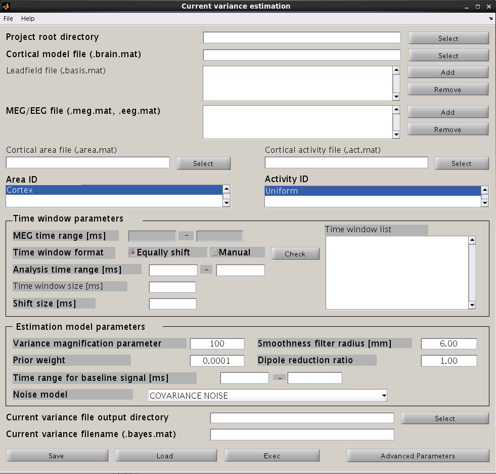
Input files
First, the cortical model file, leadfield file and MEG-MAT file have to be specified. To select leadfield file and MEG file, press the “Add” button. VBMEG can estimate the current distribution for multiple sessions at the same time. The below figure displays an example with a single session.
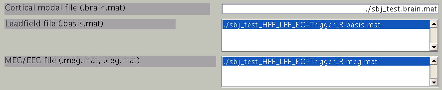
You can specify multiple leadfield/MEG-MAT files across sessions. The leadfield file and MEG-MAT file must correspond with each other: the first leadfield file is calculated from the first MEG-MAT file. The same holds for the second, third ones.
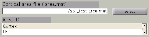
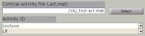
Cortical area and activity
In the next step, cortical area and cortical activity are selected. The cortical area information is used to specify the areas in which dipoles are assumed. The cortical activity information is used to determine the hyper parameters. In case you are importing fMRI data with VBMEG, it is recommended to label the cortical areas and the related activity according to the conducted MEG study. The standard cortical area ("Cortex") and cortical activity ("Uniform") are registered without fMRI data.
The cortical area ID ”Cortex” includes all vertices of the cortical model; when ”Cortex” is selected dipoles are assumed at all vertices of the cortex. The cortical activity ID ”Uniform” assumes that the whole cortex activation follows a uniform pattern. If no fMRI data is given, the cortical area ID “Cortex” will be used for the estimation with the cortical activity ID “Uniform”. Here we have imported fMRI data, so cortical activity ("LR") is used to determine hyper parameters.
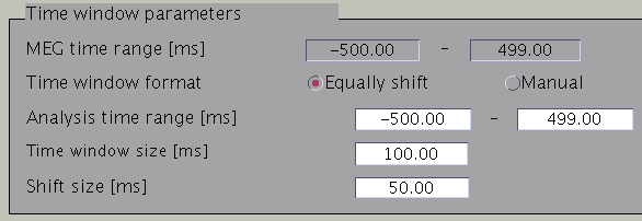
Time window parameters
VBMEG divides the MEG data into time windows of suitable length and estimates the current distribution separately for each of these windows. Based on the MEG-MAT file specified, the default parameters in the ”Time window parameters” sections will automatically be set to the default values. In the default setting, a single time window covers the whole time series. That is to say, the prior distribution of the current is assumed to be the same at each time point.
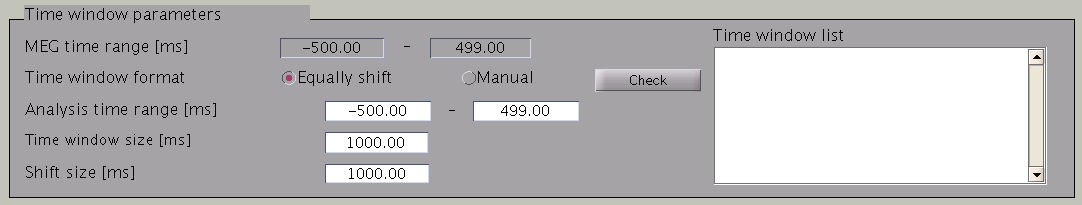
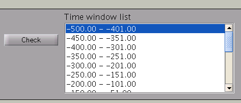
Time windows separation is favorable in case the cortical activity changes in location with time (Shibata et al., 2008, Callan et al., 2010). To divide the time window, two options are available: you can either set time window width and window shift (equally shift) or manually set every time window (manual). The two options can be selected with the ”Time window format” check box. In case of multiple time windows, window width and time shift have to be set accordingly. In our example, the MEG data was divided into 100 ms time windows. The ”Shift size” is set to 50 ms, i.e. the windows overlap 50 ms. In the overlapping regions, the current distribution is estimated independently. However, the current itself will be estimated as the average over the estimations for each window.
Pressing the ”Check” button returns a list of the individual time windows.
Estimation parameters
The figure below shows how the estimation parameters in the GUI should be set.
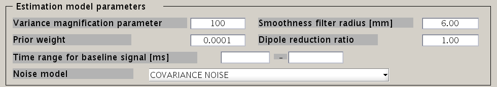
VBMEG has the following estimation parameters:
- Smoothness filter radius: VBMEG makes use of a smoothing filter that can be described by exp(-(d/R)^2), where d is the distance between two vertices measured along the cortical surface and R is the “Smoothness filter radius”. The standard value for R is 6mm.
- Dipole reduction ratio: In case the number of vertices in the cortical model should be too high, it can be reduced by setting the value for ”Dipole reduction ratio”, e.g. for a cortical model with 10,000 vertices, setting the Area ID to ”Cortex” and ”Dipole reduction ratio” to 0.2, will reduce the number of dipoles left over to 2,000.
- Noise model parameters: The standard for the ”Noise estimation model” is ”COVARIANCE NOISE”. The time interval set in ”Time range for baseline signal” determines which part of the MEG data. VBMEG uses to estimate 1) the covariance matrix of the observation noise and 2) the baseline current variance. Usually, this time interval is set as the baseline interval (time before trigger onset).
- Hyper parameters: In the hierarchical Bayesian estimation, two hyper parameters control the current estimation, the “Variance magnification parameter” (in the following referred to as m0) which controls the current strength and the ”Prior weight parameter” (in the following w0), confidence of prior information relative to data samples.
- m0 : The higher the value of m0, the higher the power of the current is estimated. In standard cases a value of m0 = 10~100 (default value = 100) is recommended.
- w0 : This value ranges from 0 to 1. w0 = 0.1 means that current variance is updated with weighted summation of prior information and data with weight 0.1 and 0.9. Setting of the prior weight depends on how reliable your prior information is. If fMRI data is available, the standard value for the prior-weight parameter w0= 0.1. The highest confidence w0=1 results in the Wiener filter estimation (Kajihara et al., 2004). If no fMRI data is available, set w0=0.0001 with act_key = 'uniform'. This results in a sparse current source image.
Output file
Finally, select the ”Current variance file directory” and the ”Current variance filename”, where the results will be stored. Note that "Current variance file" does not include current time course, but consists of current variances and other model parameters, from which the inverse filters are calculated.

After having set the parameters, press the ”Exec” button to start the estimation.
Current timecourse estimation
- VBMEG function: vb_job_current
Cortical current time course can be calculated by multiplying the inverse filters, obtained using the estimated current variance and other model parameters. This calculation can be performed by following the steps below:
- From the project manager menu, select [Analysis]->[Estimate current]. The "Current estimation" GUI will pop up.
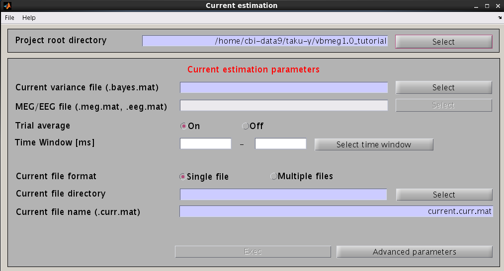
- Specify the files and parameters required.
- Specify current variance file (.bayes.mat). GUI will automatically put M/EEG-MAT file (.meg.mat/.eeg.mat) from which current variance was estimated. You can overwrite this parameter.

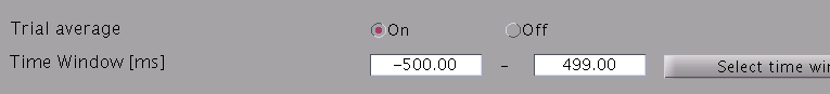
- Specify estimation parameters. If "Trial average" is "On", current timecourses are calculated for MEG data averaged across trials. You also can set a time window shorter than one used in the "Current variance estimation". By default, the time window covering whole data is used.
- Specify how to store the body of current timecourse data. If the "Single file" option is selected, estimated current time courses for all trials are saved into a single file, while if the "Multiple files" option is selected, current time courses are saved into different files for each trial.

- Specify the directory to which the cortical current file is saved. The filename is automatically set using current variance filename.

- Specify current variance file (.bayes.mat). GUI will automatically put M/EEG-MAT file (.meg.mat/.eeg.mat) from which current variance was estimated. You can overwrite this parameter.
- Press "Exec" button to start estimation of cortical current time course.
The estimated current timecourse is then saved into a cortical current file (.curr.mat).
Showing estimated source currents
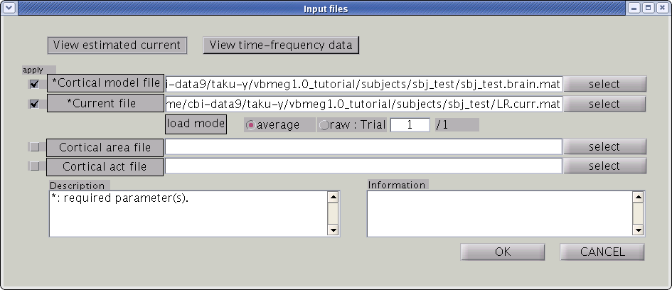
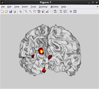
To look at the estimated cortical current, select [Tools]->[View estimated current] from the project manager menu. Then file select dialog will pop up. You need to specify the cortical current file and the cortical model file. The cortical currents will be mapped on to the cortical surface model. If you specify VBMEG AAL-area file (_aal.area.mat) or VBMEG Brodmann-area file (_brodmann.area.mat) to the Cortical area file, you can also see anatomical labels and area.
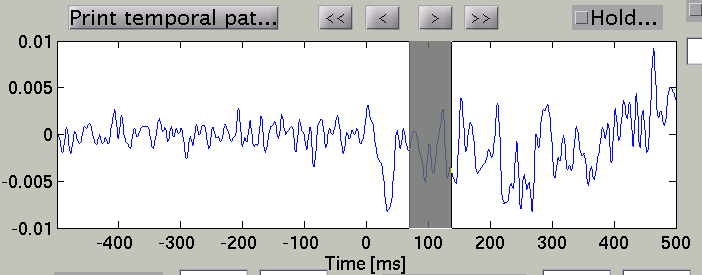
GUI of the cortical current viewer will pop up. In the left, the selected cortical surface model is plotted. The time course on the bottom is the estimated current of the selected vertex. Just after launching the GUI, the 1st vertex is selected ("Vertex number" edit box). The selected vertex is marked by a green cross (left hemisphere in the figure).
Screen description
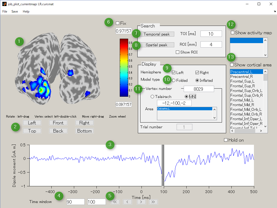
- Current map
Displays cortical model and spatial pattern of cortical current averaged over the selected time window.You can rotate in any directions by dragging the left mouse on the cortical model.
- Change viewpoint button
Select accordingly to the desired viewpoint of cortical map.
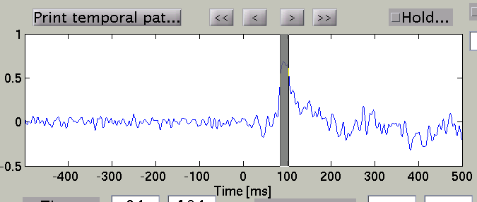
- Current timeseries and time window
This graph displays the current timeseries of the selected vertex. You can select the time window by left-dragging the mouse on this graph which is shown in a gray colored band.
- Time window
It is an interface that displays and specifies a time window for averaging current time series.
- Time window shift button
These buttons are used to move the time window.
- Current threshold for display
Specifies the current threshold value to display the boxes above and below the color bar. Normally, this threshold is automatically determined, but if you check the Fix box, the threshold is fixed.
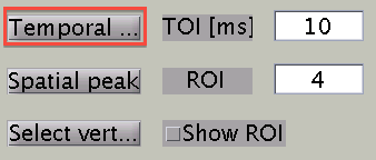
- Temporal peak button
This button is used to find the peak of time course within a specified time window (TOI[ms]).
- Spatial peak button
This button is used to find the peak of the spatial pattern within the radius of the specified ROI [mm]. Press it several times.
- Hemisphere
This is used to switch the display of the right brain / left brain.
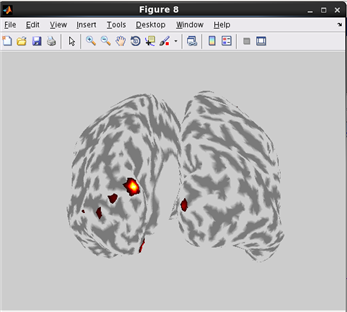
- Model type
This is used to switch the display of cortex model(Folded/Inflated). The default is Inflated.
- Vertex number
Displays the selected vertex number. On the Current map, it is displayed in green cross. It also displays the Tarairach coordinates and MNI coordinates of the selected vertices. If VBMEG area file (.area.mat) is specified, the name of the area to which the selected vertex belongs can also be displayed. For area file, if you specify AAL area file (_aal.area.mat) or Brodmann area file (_brodmann.area.mat), a generic anatomical label name will be displayed.
- Show activity map
If the VBMEG Cortical activity file (.act.mat) is specified, the activity name is displayed in the list box. If you check this box and select the activity name in the list box, the activity is displayed on the Current map. Multiple selections are possible by holding down the CTRL button and clicking the activity name.
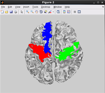
- Show cortical area button
If the VBMEG Cortical area file (.area.mat) is specified, the name of the area is displayed in the list box. If you check this box and select a region name in the list box, the area is displayed on the Current map. Multiple selections are possible by holding down the CTRL button and clicking the name of the area.
Rotate cortical model
Push "Right" button to change the viewpoint observe the cortical surface model from right.
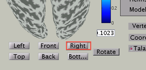
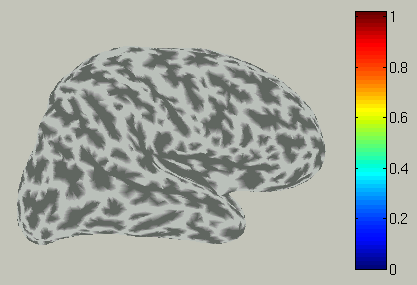
You can also rotate in any direction by dragging the left mouse button on the cortical model.
Choose hemisphere
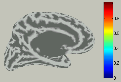
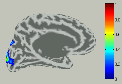
You can choose which hemisphere to be shown. To suppress the right hemisphere plot, uncheck the "Right" check box.
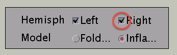
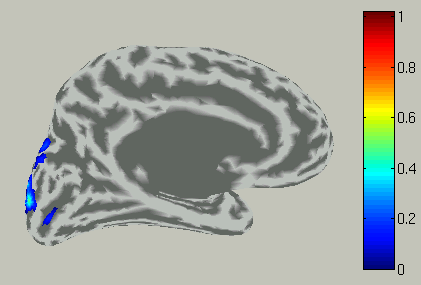
The the right hemisphere will disappear and the left hemisphere is shown in the medial view.
Choose time of interest
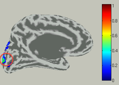
In the time course plot, you can specify an arbitrary time window by dragging the mouse on the graph. Here, the latency (about 100 ms) of the visual evoked field is selected.
Accordingly, the spatial pattern of the cortical current is shown with averaging across the time window.
View current timecourse and vertex infomation on specific vertex
To choose a vertex (current dipole), left-double-click on a point of the cortical surface model.
Then the green cross moves to the point specified,
and the timecourse plot and vertex information is changed to the one on the selected vertex.
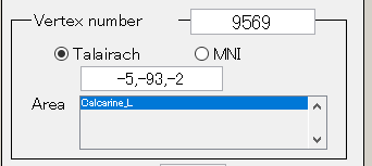
Talairach/MNI coordinate value can be switched with the radio buttons. If AAL-area file (_aal.area.mat) or Brodmann-area file (_brodmann.area.mat) is specified to Cortical area file, the label name is also displayed(e.g. Calcarine_L).
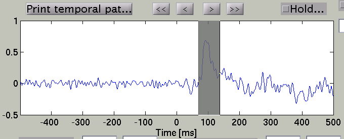
Search Temporal peak
By pressing "Temporal peak" button, you can find the peak of the timecourse within the time window.
The width of the time window after the temporal peak search is in the "TOI" editbox.
The spatial pattern of the cortical current is also updated reflecting the update of the time window.
8.Connectome dynamics
Connectome dynamics estimation is a new approach to estimate current source dynamics model by using whole-brain anatomical connectivity information (connectome) extracted from diffusion MRI. In this section, we will explain how to process dMRI data, two types of dynamics estimation, and how to create a dynamics movie using VBMEG ver 2.0. It is assumed that preprocessing of Source imaging (brain modeling, MEG data preprocessing, fMRI data preprocessing, and leadfield calculation) has been completed.
As shown below, two ways to estimate connectome dynamics are implemented; simultaneous current and dynamics estimation proposed in Fukushima et al. 2015, two-step estimation where current source imaging is followed by connectome dynamics estimation via l2-regularized least square method. Ideally the former is superior to the latter because source imaging is estimated with connectome dynamics information but we have found a critical issue called a waveform distortion problem in which a part of current source waveform showed unrealistic drift-like behavior. Since we have not fixed it yet, we highly recommend the two-step method for real data analysis in practice for now.
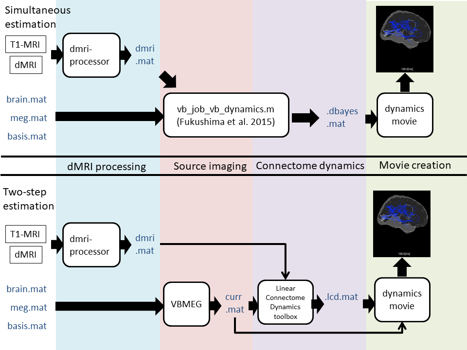
To obtain an individual subject's connectome from diffusion MRI data with high-angular resolution (typically more than 64 in our lab), probabilistic tractography with spherical deconvolution implemented in MRtrix is used. Then connectome dynamics is estimated from the obtained connectome and current source time courses. Finally dynamics movie is created with the estimated connectome dynamics model.
Diffusin MRI data processing
Dynamics estimation
- Linear Connectome Dynamics estimation : Two-step method
- Fukushima's dynamics estimation (under construction, Japanese only)
Dynamics movie
- Connectome dynamics movie (under construction)
A-1.VBMEG APIs
Data Import functions
| vb_job_brain | Converts FreeSurfer data to VBMEG format. |
| vb_job_head_3shell | Makes 1-shell(CSF) for MEG or 3-shell(CSF, Skull, Scalp) surface model for EEG. |
| vb_job_fmri | Imports fMRI activities as a prior information. |
| vb_job_meg | Imporst M/EEG data and creates VBMEG MEG (.meg.mat) or EEG (.eeg.mat) file. |
Source Imaging functions
| vb_job_leadfield | Calculates leadfield matrix for using the numerical methods. |
| vb_job_vb | Computes current variance from the M/EEG data using hierarchical Bayesian method. |
| vb_job_current | Calculates cortical current from the estimated current variance and M/EEG data. |
Data Load functions
| vb_load_cortex | Loads cortical model of standard brain. |
| vb_load_current | Loads estimated cortical current of standard brain. |
| vb_load_channel | Loads channel position for plotting M/EEG data. |
| vb_load_meg_data | Loads M/EEG data. |
| vb_load_sensor | Loads sensor position for computing leadfield. |
| vb_get_keyset_area | Gets a list of keys for Cortical area. |
| vb_get_area | Loads area data. |
| vb_get_keyset_act | Gets a list of keys for Cortical activity. |
| vb_get_act | Loads activity data. |
Data Plot functions
| vb_plot_cortex | Plots cortex and current. |
| vb_plot_area | Plots cortical area map. |
| vb_plot_sensor_2d | Plots a topographic map of M/EEG field as a 2D field. |
A-2.Tips
how to plot current on cortical model. (Code)
related functions:vb_plot_cortex, vb_load_cortex
how to plot current on Inflated cortical model.(Code)
related functions:vb_plot_cortex, vb_load_cortex
how to plot cortical map on cortical model.(Code)
related functions:vb_plot_area
how to plot cortical map on Inflated cortical model.(Code)
related functions:vb_plot_area
how to plot a topographic map of M/EEG data.(Code)
related functions:
vb_plot_sensor_2d, vb_load_channel, vb_load_meg_data
What is gray matter file and SPM normalization file?
Gray matter file and SPM normalization file are used for the following purposes.
- Gray matter file(c1*.nii)
- This is used as a mask so that head model does not intrude into the cortex.
- SPM normalization file(*_sn.mat)
- This is used to unnormalize fMRI activities analyzed on standard brain to an individual brain.
These files can be created by Segment function of SPM8.
- SPM8 Segment GUI
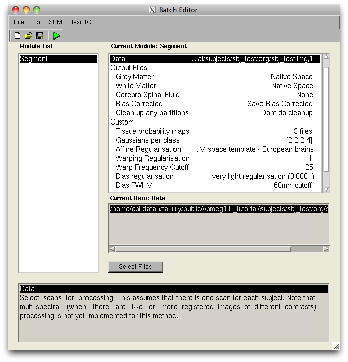
- VBMEG function for calling SPM Segment function
It can be used the Segment function of SPM8 from the VBMEG function.
- Function name
- vb_sn_and_graymatter_file_create
- Description
- Create gray matter file(c1*.nii) and SPM normalization file(*_sn.mat) from the specified MRI file. They are created in the same directory as the original file.
- Syntax
- vb_sn_and_graymatter_file_create(mri_file);
- Parameters
- mri_file : NIfTI file(.nii)
- Output files
- 1.Gray matter file(c1*.nii)
2.SPM normalization file(*_sn.mat)
- Remarks
- SPM8 should be added to your MATLAB(e.g. addpath(genpath('SPM8path'))
How to change project directory?
To transfer the directory, simply copy the entire project directory and change the proj_root in the project file(.prj.mat) as below and you can restart the analysis.
>proj_root = 'new_proj_root';
>vb_save(project_file, 'proj_root');
What is the unit of cortical current estimated with VBMEG?
- By default, the unit of cortical current is Ampere meter (Am). If patch normalization is applied during estimation, the unit is Am/m^2. As a supplement, all physical variables of VBMEG have standard SI units (e.g., MEG signals have "Tesla" as its unit as opposed to pico/femto Tesla). The same holds for the cortical current.
Which direction does estimated cortical current at each vertex flow?
- In cortical current files (.curr.mat), a positive current is defined as one directed toward the outside of the cortex. However, the direction is automatically flipped when plotting cortical currents by job_plot_currentmap; current directed toward the inside of the cortex is shown as positive.
Which kind of information does positioning files (.pos.mat) include?
- Positioning files include a 4-by-4 affine transformation matrix (trans_info, obtained by vb_posfile_get_transinfo.m). The affine matrix transforms the sensor coordinate system (position and direction) in the hardware space (measurement system dependent) to the 'SPM_Right_m' space (MRI dependent).
How do I get axial sensors of Yokogawa MEG system?
- You can use VBMEG function vb_load_channel_info:
>> [pos, ch_info] = vb_load_channel('your_meg_file.meg.mat');
'ch_info' is a struct including information of sensors.
>> ch_info

ch_info =

    Active: [400x1 double]
      Name: {400x1 cell}
      Type: [400x1 double]
        ID: [400x1 double]
'ch_info.Type' includes sensor type. In Yokogawa MEG system at ATR with 400 channels, 2 and 3 indicate axial and planar sensors, respectively. Indices of axial sensors can be obtained with the following code:
ix_axial = find(ch_info.Type==2);
How do I get the nearest neighbors to a vertex?
The cortical model file includes distances from each vertex to neighbors. The following code is an example to get neighbors to a vertex within 10mm radius.
[nextDD,nextIX] = vb_load_cortex_neighbor('your_brain_file.brain.mat');
ix_center           = 100; % center of ROI
ixx                    = find(nextDD{ix_center}<=10e-3);
ix_roi                = nextIX{ix_center}(ixx); % ix_roi is the set of vertices within 10mm from ix_center
How do I make my own fMRI prior?
You may want to combine two or more fMRI prior to estimate cortical current during multiple conditions but with the single prior. The following code is an example to calculate average of cortical activity data already stored and store the averaged activity data to a cortical activity file.
act_file1 = 'your_act_file1.act.mat';
act_file2 = 'your_act_file2.act.mat'; % this can be the same with act_file1.

act1 = vb_get_act(act_file1,'act_key_cond1');
act2 = vb_get_act(act_file2,'act_key_cond2');

act_new.xxP = (act1.xxP+act2.xxP)./2;
act_new.key = 'act_key_new'; % ID of new activity map

vb_add_act(act_file2,act_new); % store new activity map
The average activity map will be stored in act_file2 with ID 'act_key_new'.
Add new area information into cortical area file (.area.mat)
Extract an area on which some activities (e.g., t-value) are larger than a threshold
% files and ids
area_file = 'sbj.area.mat';
act_file = 'sbj.act.mat';

% thresholding
act = vb_get_act(act_file,'t_value'); % get activity map 't_value' stored in act_file
ix = find(a.xxP>=threshold);

% make and add new area
area_new.Iextract = ix; % thresholded area
area_new.key = 'area_new_id';  % any identifier
vb_add_area(area_file,area_new); % area_new is added to area_file
Concatenate two areas (union)
% files
area_file = 'sbj.area.mat';

% get areas
area1 = vb_get_area(area_file,'area1');
area2 = vb_get_area(area_file,'area2');

% concatenation
ix = union(area1.Iextract,area2.Iextract);

% make and add new area
area_new.Iextract = ix;
area_new.key = 'area_new_id';  % any identifier
vb_add_area(area_file,area_new); % area_new is added to area_file
How to improve data saving/loading time performance?
If you speed up saving/loading time, we recommend to use -v6 MAT-file format with cost of slight increase of file size. Detailed information on MATLAB save options can be found here(Undocumented Matlab). Note that -v6 option has limitation on memory size of one variable in a file (maximum 2GB/variable). There are two ways to change the save format.
- By changing MATLAB setting

This setting affects other programs. If you want to avoid it, please use VBMEG command. - By using VBMEG command
You can temporarily change the format on VBMEG. If you exit MATLAB or execute 'clear global' command, the affect disappers.
vbmeg('save_version', '-v6');
or
vbmeg('save_version', '-v7.3');
As default setting, VBMEG saves data in file format according to MATLAB settings.
A-3.Troubleshooting
How to resolve the error Output argument z (and maybe others) not assigned during call to vb_repmultiply.m?
- You need to recompile MEX-files for your system. It can be done just by running following functions.
- vb_mex_compile.m
- vb_mex_compile_utilities.m
How to resolve the error Invalid MEX-file (mexfilename) The specified module could not be found. on Windows?
- You need to install Microsoft Visual C++ 2010 Redestributable Package (x86/x64) on your system. see the following URLs.
- for x86: vcredist_x86.exe: http://www.microsoft.com/en-us/download/details.aspx?id=5555
- for x64: vcredist_x64.exe: http://www.microsoft.com/en-us/download/details.aspx?id=14632
A-4.References
- Yoshimura, N., Tsuda, H., Kawase, T., Kambara, H., Koike, Y.,(2017), Decoding finger movement in humans using synergy of EEG cortical current signals, Scientific Reports, 7, Article 11382
- Yanagisawa, T., Fukuma, R., Seymour, B., Hosomi, K., Kishima, H., Shimizu, T., Yokoi, H., Hirata, M., Yoshimine, T., Kamitani, Y., Saitoh, Y., (2016), Induced sensorimotor brain plasticity controls pain in phantom limb patients, Nature Communications, 7, Article 13209
- Callan, D.E., Terzibas, C., Cassel, D.B., Sato, M., Parasuraman, R., (2016), The brain is faster than the hand in split-second intentions to respond to an impending hazard: a simulation of neuroadaptive automation to speed recovery to perturbation in flight attitude. Frontiers in Human Neuroscience, 10, Article 187
- Fukushima, M., Yamashita, O., Knoesche, T.R., Sato, M., (2015), MEG source reconstruction based on identification of directed source interactions on whole-brain anatomical networks. NeuroImage, 105, 408-427
- Toda A, Imamizu H, Kawato M, Sato MA.(2011). Reconstruction of two-dimensional movement trajectories from selected magnetoencephalography cortical currents by combined sparse Bayesian methods. NeuroImage. 54(2), 892-905.
- Yoshimura, N., Dasalla, C. S., Hanakawa, T., Sato, M., Koike, Y., (2011). Reconstruction of flexor and extensor muscle activities from electroencephalography cortical currents. NeuroImage, 59, 2, 1324-1337 .
- Sato, M., Yoshioka, T., Kajiwara, S., Toyama, K., Goda, N., Doya, K., & Kawato, M. (2004). Hierarchical Bayesian estimation for MEG inverse problem. NeuroImage, 23, 806–826.
- Kajihara S, Ohtani Y, Goda N, Tanigawa M, Ejima Y, Toyama K. (2004). Wiener filter-magnetoencephalography of visual cortical activity. Brain Topogr. 2004 Fall;17(1):13-25.
- Mackay, D.J.C, (1992), Neural computation, 4, pp.415-447;
A-5.Acknowledgement
- Funding
This software development is supported by contract research from the National Institute of Information and Communications Technology, Japan (grant #136 #173).
- Tools
- FreeSurfer
- SPM
- MRtrix
- FSL
- EEG 10-20 coordinates from Prof.Dan (Chuo University)
Last update: 2018/04/11