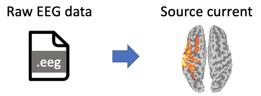
Source imaging only from EEG data
Contents
1. Introduction
1.1. Scenario
Generally, source imaging from EEG data requires the information of a subject’s brain structure and EEG sensor locations, which are respectively obtained using MRI system and 3D scanner. However, the MRI system and 3D scanner are expensive equipment and not many facilities have access to them. It is a common case that we only have EEG data but want to conduct the source imaging. Indeed, VBMEG provides a solution for such case by substituting the subject’s brain structure and EEG sensor locations with the standard models. In this tutorial, we demonstrate this solution using the real experimental data. All the procedures will be conducted with scripts.
1.2. Experimental procedure
In the experiment, the subject performed a somatosensory task. The subjects were instructed to close their eyes and an electrical stimulation was presented to the right median nerve. During the experiment, EEG was recorded with a whole-head 63-channel system (BrainAmp; Brain Products GmbH, Germany).
2. Starting tutorial
2.1. Setting environment
This tutorial was developed using MATLAB 2019a with Signal Processing Toolbox on Linux.
(1) Download and unzip tutorial.zip
(2) Copy and paste all the files to $your_dir
(3) Start MATLAB and change current directory to $your_dir/program
(4) Open make_all.m by typing
>> open make_all
2.2. Adding necessary toolboxes to search path
Thereafter, we will sequentially execute the commands in make_all.m from the top.
We add the VBMEG toolbox to search path. Please modify this for your environment.
>> path_of_VBMEG = '/home/cbi/takeda/analysis/toolbox/vbmeg_20220721';
>> addpath(path_of_VBMEG);
>> vbmeg
2.3. Set parameters
We set the parameters for analyzing the EEG data, and set the file and directory names.
>> sub = 's006';
>> p = set_parameters(sub);
You can also set sub = 's043'.
By default, analyzed data and figures will be respectively saved in
- $your_dir/analyzed_data/s006,
- $your_dir/figure.
3. Source imaging only from EEG data
In this section, we introduce the procedures from importing the raw EEG data to the source current estimation.
3.1. Preprocessing
Importing EEG data
We convert BrainAmp files to MAT files (User manual, vb_job_meg.m).
>> import_eeg(p);
The following file will be saved.
- $your_dir/analyzed_data/s006/loaded/s1.eeg.mat (Somatosensory task, run 1)
Filtering EEG data
The recorded EEG data include drift and line noise (60 Hz at Kansai in Japan). To remove these noises, we apply a low-pass filter, down-sampling, and a high-pass filter.
>> filter_eeg(p);
The following file will be saved.
- $ your_dir/analyzed_data/s006/filtered/s1.eeg.mat
Making trial data
We segment the continuous EEG data into trials. First, we detect stimulus onsets from the trigger signals included in the EEG data. Then, we segment the EEG data into trials by the detected stimulus onsets.
>> make_trial_eeg(p);
The following file will be saved.
- $your_dir/analyzed_data/s006/trial/s1.eeg.mat
Removing EOG components
We regress out EOG components from the EEG data. For each channel, we construct a linear model to predict the EEG data from the EOG data and remove the prediction from the EEG data.
>> regress_out_eog_from_eeg(p);
The following file will be saved.
- $your_dir/analyzed_data/s006/trial/r_s1.eeg.mat
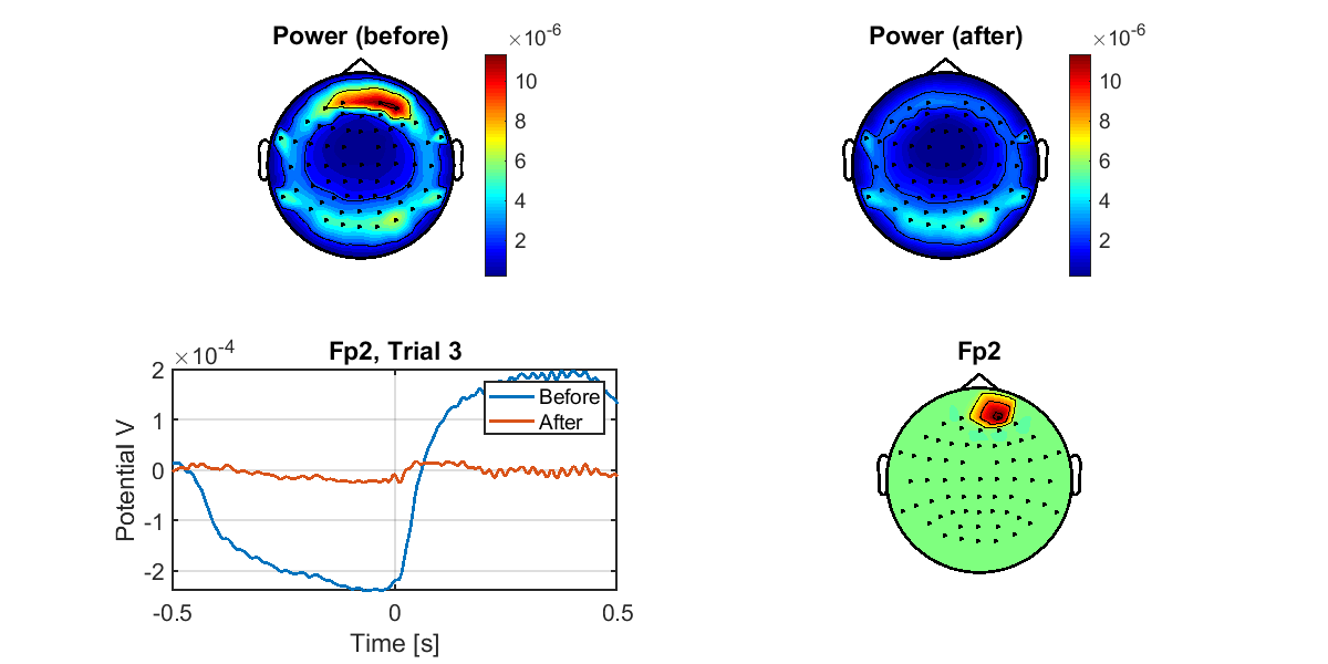
Checking the result of removing EOG components
To check if the EOG components were correctly removed, we compare the spatial distributions of the powers between the original and the EOG-removed EEG data (vb_plot_sensor_2d.m).
>> check_removing_eog_from_eeg(p);
The following figure will be saved.
- $your_dir/figure/check_removing_eog_from_eeg/s006.png
Correcting baseline
For each channel and trial, we make the average of prestimulus EEG to 0.
>> correct_baseline_eeg(p);
The following file will be saved.
- $your_dir/analyzed_data/s006/trial/br_s1.eeg.mat
Applying independent component analysis (ICA)
Using EEGLAB, we apply ICA to the EEG data.
>> apply_ica_eeg(p);
The following file will be saved.
- $your_dir/analyzed_data/s006/ica/apply_ica_eeg.mat
Automatically classifying ICs
We automatically classify each IC into brain activities and noise based on its kurtosis, entropy, and stimulus-triggered average (Barbati et al., 2004).
>> classify_ic_eeg(p);
The following file will be saved.
- $your_dir/analyzed_data/s006/ica/classify_ica_eeg.mat
Showing ICs
For each IC, we show its spatial pattern, stimulus-triggered average, and power spectrum. For the ICs classified as noise, their stimulus-triggered averages and power spectra were shown by red lines.
>> show_ic_eeg(p);
Figures will be saved in
- $your_dir/figure/show_ic_eeg/s006.
Removing noise ICs
We remove the ICs classified as noise from the EEG data (Jung et al., 2001).
>> remove_noise_ic_eeg(p);
The following file will be saved.
- $your_dir/analyzed_data/s006/trial/ibr_s1.eeg.mat
Taking common average
We take common average; that is, we make the averages of EEG data across the channels to 0.
>> common_average_eeg(p);
The following file will be saved.
- $your_dir/analyzed_data/s006/trial/cibr_s1.eeg.mat
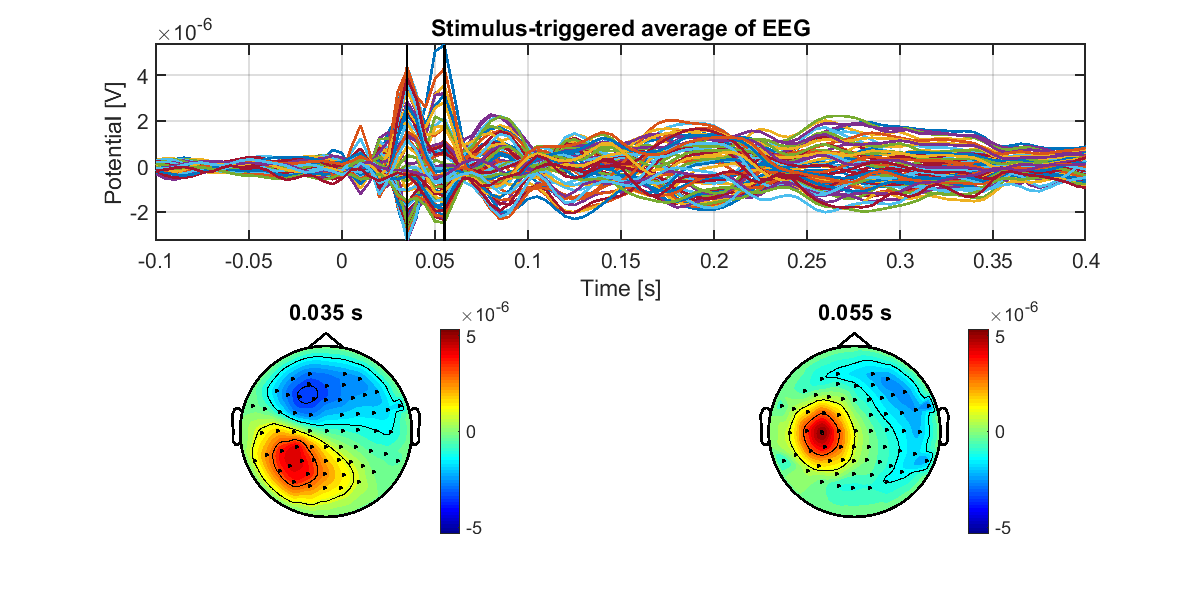
Showing preprocessed EEG data
We show the processed EEG data averaged across the trials (vb_plot_sensor_2d.m).
>> show_trial_average_eeg(p);
The following figure will be saved.
- $your_dir/figure/show_trial_average_eeg/s006.png
3.2 Source imaging
Preparing brain model
We copy the standard brain model to $your_dir/analyzed_data/s006/brain.
>> prepare_brain_model(p);
The following files will be saved.
- $your_dir/analyzed_data/s006/brain/Subject.brain.mat (Brain model)
- $your_dir/analyzed_data/s006/brain/Subject.act.mat
- $your_dir/analyzed_data/s006/brain/Subject.area.mat
Preparing leadfield
VBMEG3 provides the following leadfield matrix for the standard brain.
- mni_icbm152_t1_tal_nlin_asym_09c_10000.basis.mat
From this file, we extract the leadfield vectors corresponding to the recorded EEG channels by matching the channel names.
>> prepare_leadfield_eeg(p);
The following file will be saved.
- $your_dir/analyzed_data/s006/leadfield/Subject.basis.mat
Estimating source current
Using the leadfield matrix, we estimate the source current variance (vb_job_vb.m). Finally, the source current variance is used to yield the estimation of source current (vb_job_current.m).
>> estimate_source_current_eeg(p);
The following files will be saved.
- $your_dir/analyzed_data/s006/current/s.bayes.mat (current variance)
- $your_dir/analyzed_data/s006/current/s.curr.mat (source current)
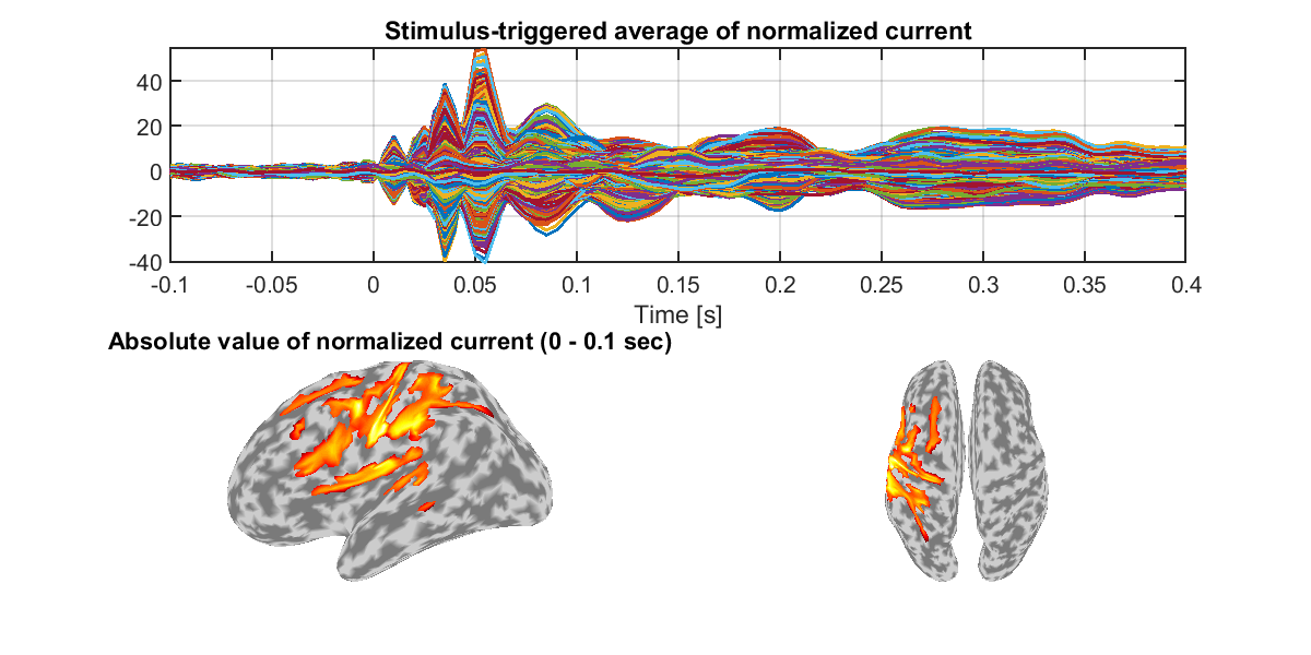
Showing estimated source current
We show the estimated source current averaged across the trials (vb_plot_cortex.m). For each source, the averaged current is normalized so that its baseline period has a mean 0 and standard deviation 1.
>> show_source_current_eeg(p);
The following figure will be saved.
- $your_dir/figure/show_source_current_eeg/s006.png
Congratulations! You have successfully achieved the goal of this tutorial.