OPM simulation test
Contents
- Contents
- 0. Download
- 1. Introduction
- 2. Starting tutorial
- 3. Simulating SQUID- and OPM-MEG data
- 4. Estimating currents
0. Download
Data and programs (opm_simulation.zip)
1. Introduction
1.1. Scenario
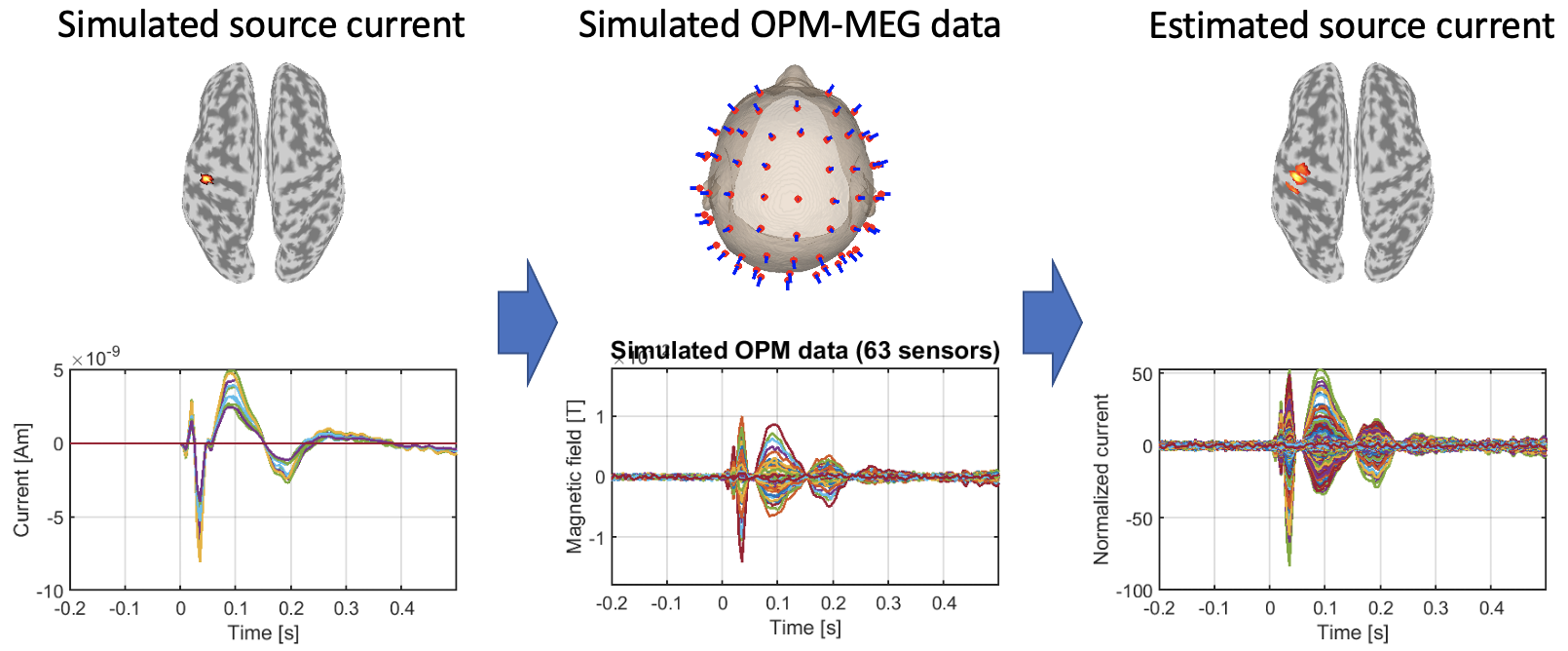
Using simulated data and VBMEG, this tutorial demonstrates the source imaging from magnetoencephalography (MEG) data recorded with a new type of MEG device, an optically pumped magnetometer (OPM). For comparison, the source imaging from simulated SQUID-MEG data will also be performed. All the procedures will be conducted with scripts.
1.2. Assumed experimental procedure
This simulation test assumes that a subject performed a somatosensory task, in which an electrical stimulation was repeatedly presented to his right median nerve.
We assume that SQUID- and OPM-MEG were respectively recorded with a whole-head 400-channel system (210-channel Axial and 190-channel Planar Gradiometers; PQ1400RM; Yokogawa Electric Co., Japan) and the QuSpin Zero-Field Magnetometer (QZFM) Gen-2 (QuSpin Inc., USA).
2. Starting tutorial
2.1. Setting environment
This tutorial was developed using MATLAB 2019a on Linux.
(1) Download and unzip opm_simulation.zip
(2) Copy and paste all the files to $your_dir
(3) Start MATLAB and change current directory to $your_dir/program
(4) Open make_all.m by typing
>> open make_all
2.2. Adding VBMEG to search path
Thereafter, we will sequentially execute the commands in make_all.m from the top.
We add the VBMEG toolbox to search path.
>> path_of_VBMEG = '/home/cbi/takeda/analysis/toolbox/vbmeg_20210518';
>> addpath(path_of_VBMEG);
>> vbmeg
You need to modify path_of_VBMEG for your environment.
2.3. Creating a project
We set the parameters for this simulation test.
>> p = create_project;
By default, generated data and figures will be respectively saved in
- $your_dir/simulated_data,
- $your_dir/figure.
3. Simulating SQUID- and OPM-MEG data
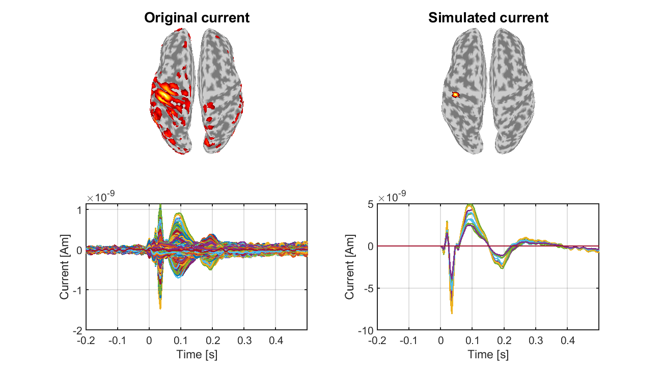
3.1. Simulating a source current
First of all, we simulate a source current based on that estimated from the real SQUID-MEG data during the somatosensory task.
>> make_sim_current(p);
The following file and figure will be saved.
- $your_dir/simulated_data/cur.mat
- $your_dir/figure/simulated_current.png
3.2. Determining OPM sensor locations
We determine the locations and directions of simulated OPM sensors. To determine the locations, we project those of the real EEG sensors on the scalp surface and move them up 8 mm from the scalp surface. The directions are set to be normal to the scalp surface. The OPM sensor information is saved in a tentative MEG file (tmp.meg.mat).
>> make_sim_pick(p);
The following file and figures will be saved.
- $your_dir/simulated_data/tmp.meg.mat
- $your_dir/figure/squid_sensor.png
- $your_dir/figure/opm_sensor.png
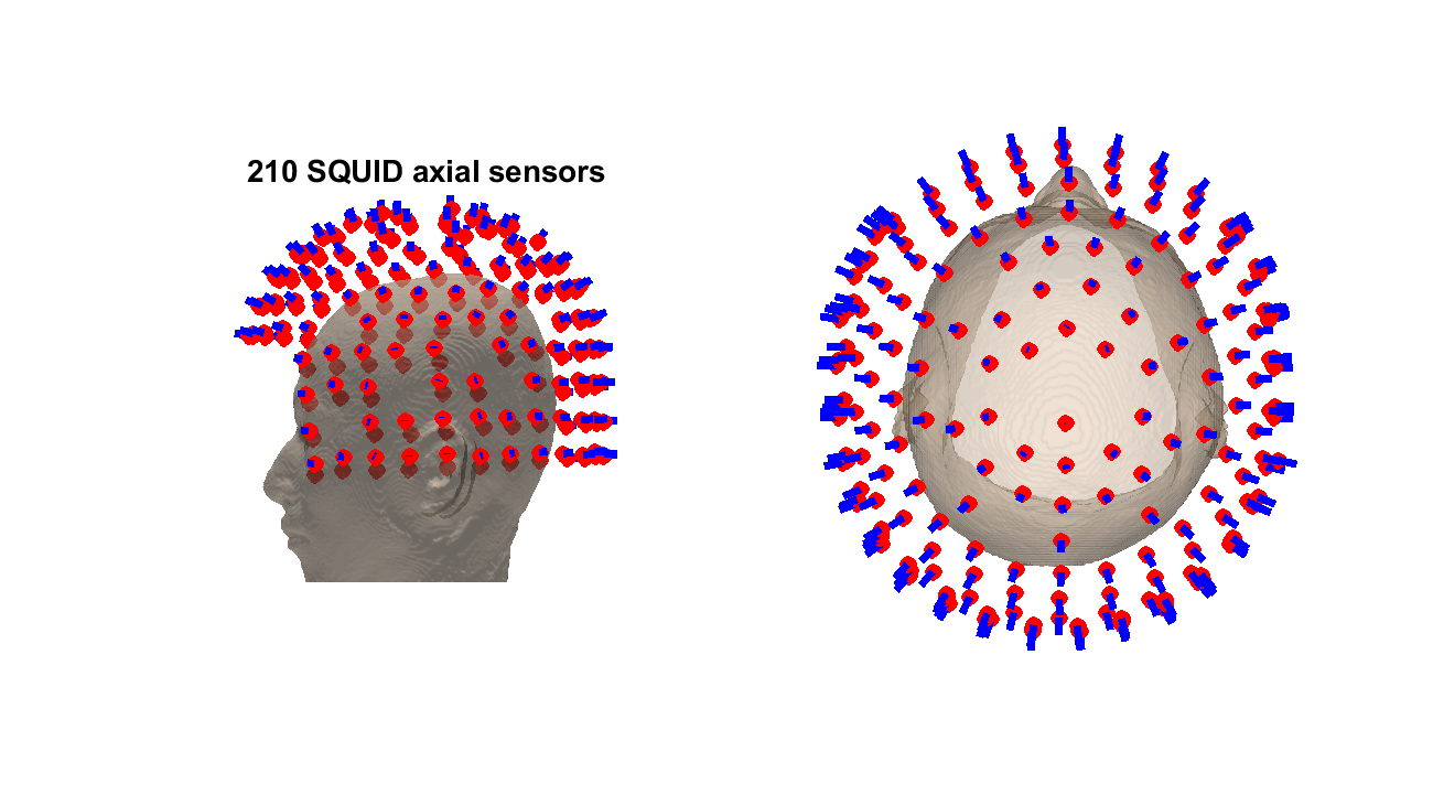
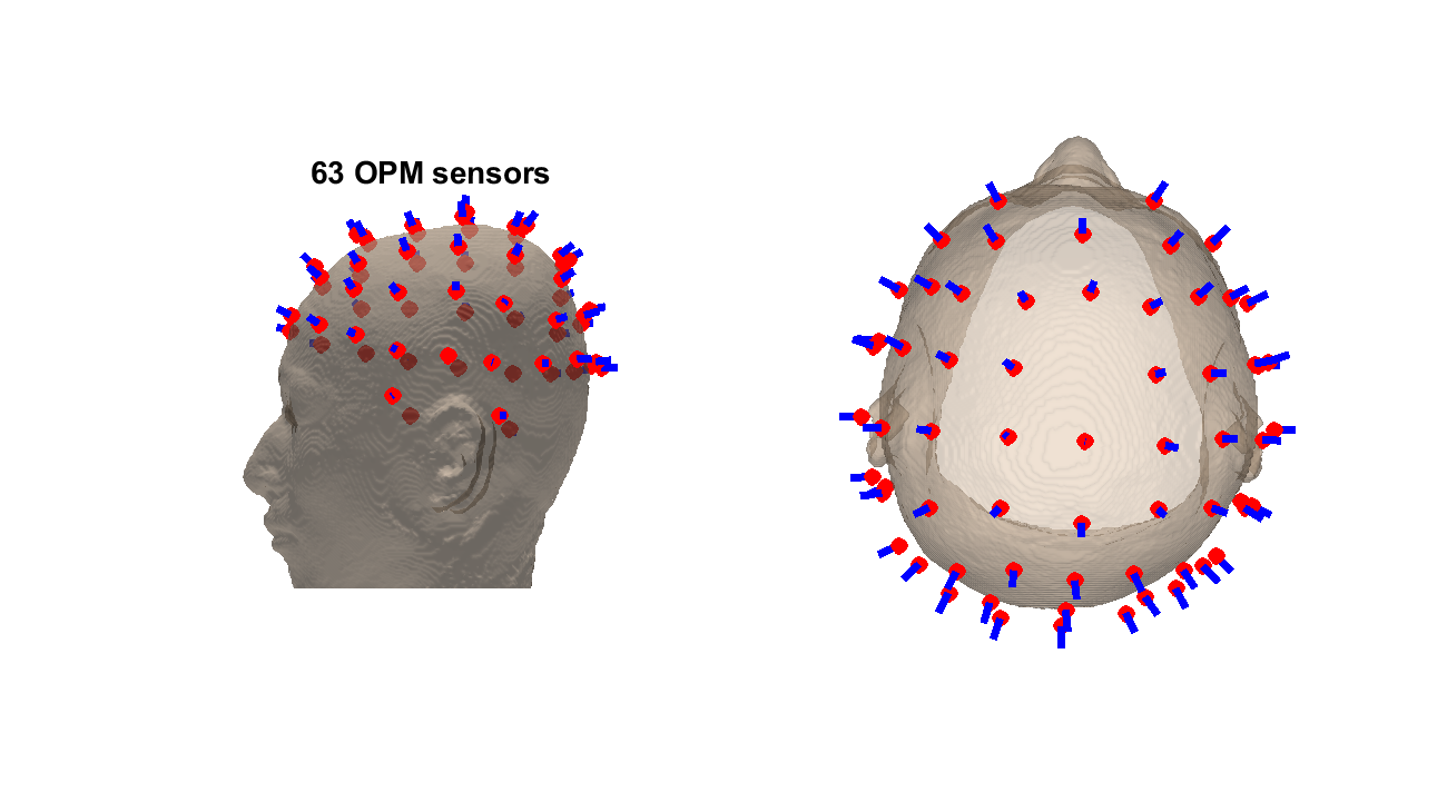
In these figures, red dots and blue lines respectively indicate the sensor locations and directions.
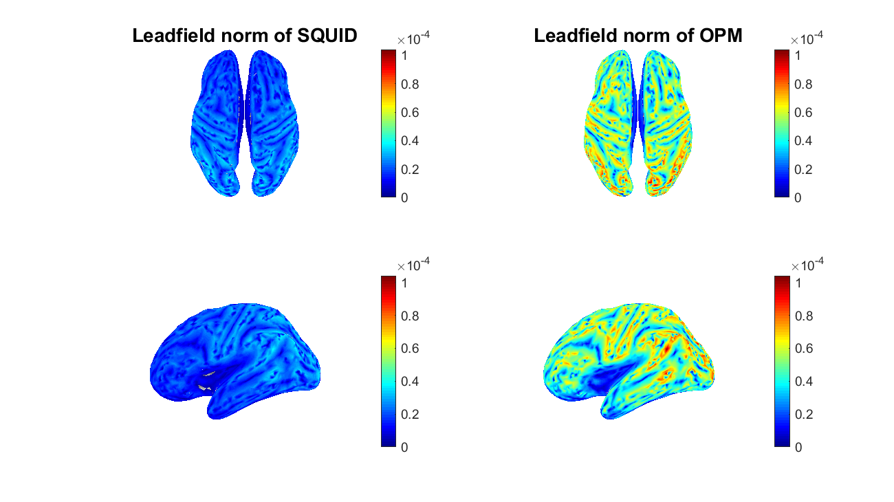
3.3. Making a leadfield matrix
We make the leadfield matrix for the OPM sensors.
>> make_sim_basis(p);
The following file and figure will be saved.
- $your_dir/simulated_data/Subject.basis.mat
- $your_dir/figure/leadfield_norm.png
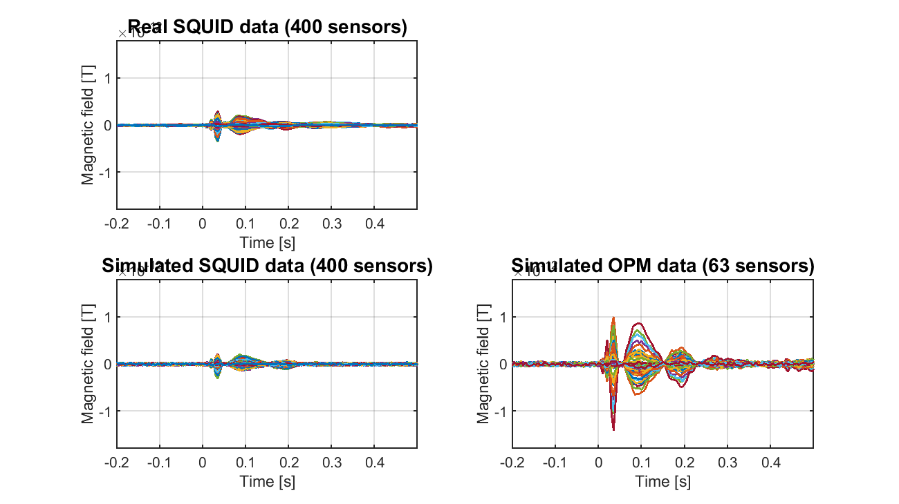
3.4. Making simulated SQUID- and OPM-MEG data
Using the leadfield matrices, we make simulated SQUID- and OPM-MEG data.
>> make_sim_meg(p);
The following files and figure will be saved.
- $your_dir/simulated_data/squid.meg.mat
- $your_dir/simulated_data/opm.meg.mat
- $your_dir/figure/simulated_meg.png
4. Estimating currents
4.1. Estimating current from SQUID-MEG data
We estimate the source current from the simulated SQUID-MEG data.
>> est_sim_current_squid(p);
The following file will be saved.
- $your_dir/simulated_data/squid.bayes.mat (current variance)
- $your_dir/simulated_data/squid.curr.mat (source current)
4.2. Estimating current from SQUID-MEG data
We estimate the source current from the simulated OPM-MEG data.
>> est_sim_current_opm(p);
The following file will be saved.
- $your_dir/simulated_data/opm.bayes.mat (current variance)
- $your_dir/simulated_data/opm.curr.mat (source current)
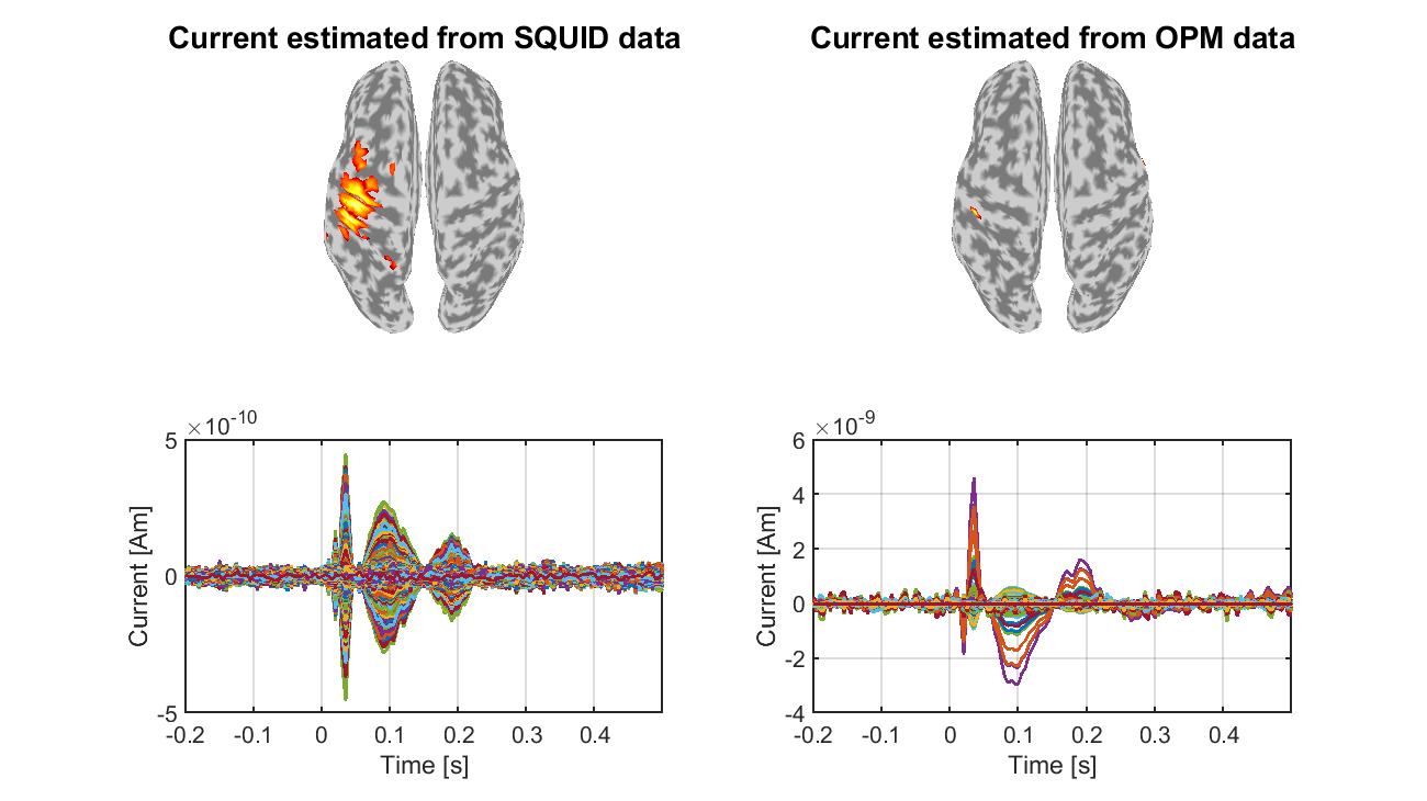
4.3. Showing estimated currents
We show the currents estimated from the simulated SQUID- and OPM-MEG data.
>> show_est_current(p);
The following figure will be saved.
- $your_dir/figure/estimated_currents.png
Furthermore, we show the currents normalized to have means 0 standard deviations 1 during a baseline period.
- $your_dir/figure/normalized_estimated_currents.png
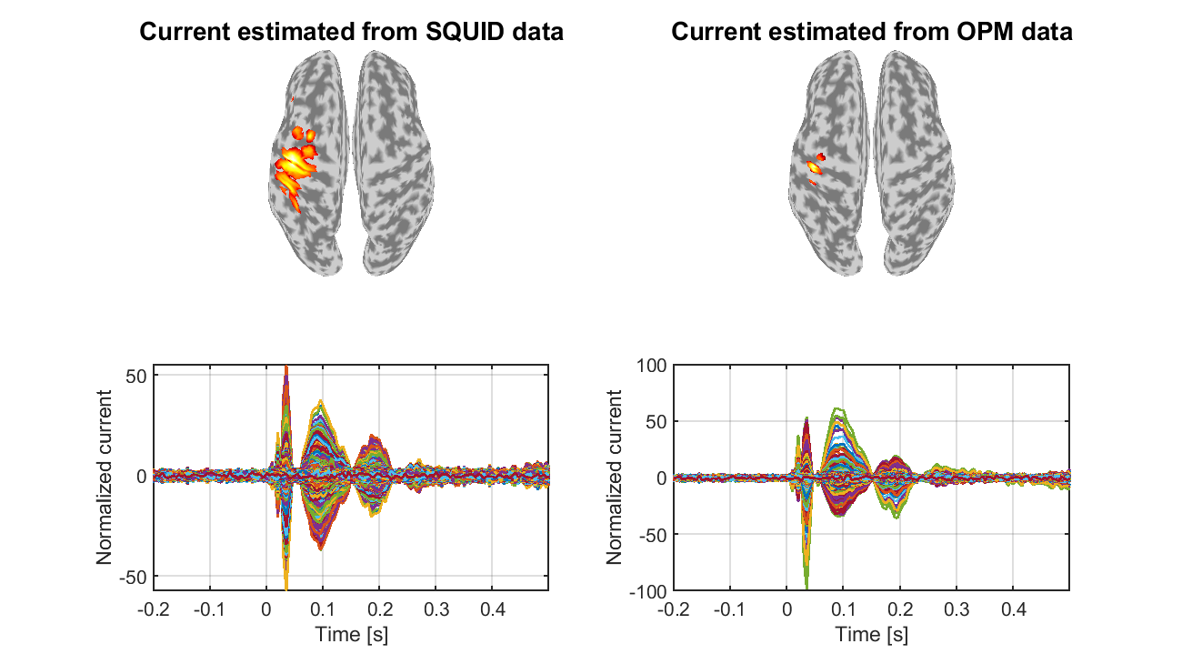
Congratulations! You have successfully achieved the goal of this tutorial.