VBMEG users manual for ver 1.0.2
- Overview
- Preparation of files required for VBMEG
- Setup and launch GUI
- Data import
- Cortical current estimation
- View cortical current
- Advanced topics
- FAQ
- What is the unit of cortical current estimated with VBMEG?
- Which direction does estimated cortical current at each vertex flow?
- Which kind of information does positioning files (.pos.mat) include?
- How do I get axial sensors of Yokogawa MEG system?
- How do I get the original vertex indices for estimation results with reduce parameter less than 1?
- How do I get the nearest neighbors to a vertex?
- How do I make my own fMRI prior?
- Troubleshooting
- How to resolve the error 'Output argument "z" (and maybe others) not assigned during call to "$VBMEG\vb_repmultiply.m>vb_repmultiply".'?
- How to resolve the error 'Invalid MEX-file <mexfilename> The specified module could not be found.' on Windows?
- The result of fMRI import looks strange. How do I fix it?
- MATLAB Scripts
- References
Overview
VBMEG is a free MATLAB toolbox that solves the M/EEG inverse problem using hierarchical Bayesian estimation (Sato et al., 2004). Using VBMEG one can:
- Import cortical surface model created by other software packages (i.e., FreeSurfer, BrainVoyager)
- Import M/EEG data (Yokogawa, Biosemi).
- Import fMRI activities (statistical parametric map) calculated with SPM2/5/8.
- Calculate M/EEG forward model (leadfield).
- Estimate M/EEG inverse filter.
- Estimate cortical current.
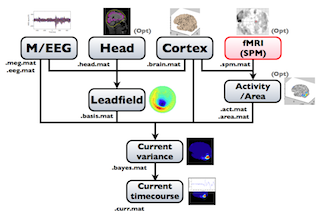
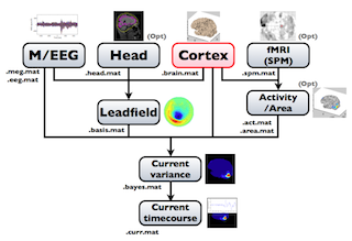
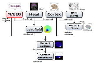
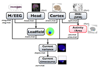
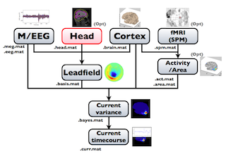
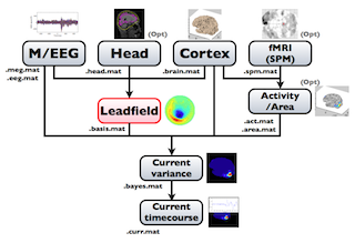
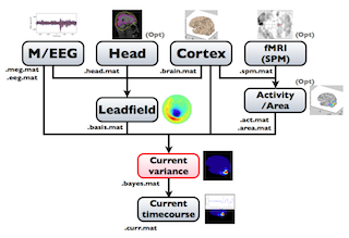
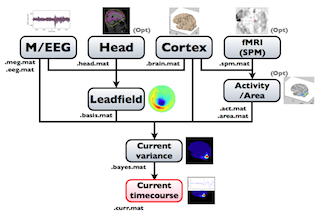
The following figure is a diagram of VBMEG processes for cortical current estimation.
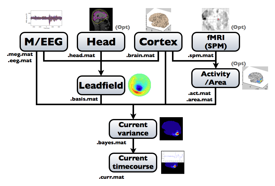
To make SPM-voxel file ("fMRI (SPM)" in the diagram), you need to invoke a VBMEG function on a MATLAB console in which SPM is running. The preprocessing ("M/EEG", "Cortex", "Head", and "Activity/Area") and analysis ("Leadfield", "Current variance", and "Current timecourse") steps can be performed on GUI.
Hardware and software requirements
- VBMEG is running on MATLAB environment (version 7.0 or later). Since some MEX-files run only on Windows XP or Linux/x86, any other operating system is not supported.
- FreeSurfer (4.2 or later) or BrainVoyager (2000/QX) are needed to create cortical surface model (gray matter/white matter boundary).
- If you want to use fMRI data as prior information for cortical current estimation, a statistical parametric map of t-values obtained with SPM2/5/8 can be incorporated into VBMEG.
- If you use BEM (boundary element method) to calculate M/EEG forward model (leadfield), Curry or SPM8 software can be used to make skull and scalp surfaces. A simple sphere model can also be used for the forward model calculation.
- The following data are required for cortical current estimation by VBMEG:
- Structural MRI data (ANALYZE/NIfTI).
- Cortical surface model (FreeSurfer/BrainVoyager).
- M/EEG data (Yokogawa/Biosemi).
- Positioning data (Fastscan).
- fMRI data (SPM8; optional).
- Head model (SPM8 and FreeSurfer/Curry; optional).
VBMEG file type
The following files are created by VBMEG:
- Cortical surface model file (.brain.mat) a polygon model of gray/white matter boundary, inflated model for displaying purposes, and information related to the model.
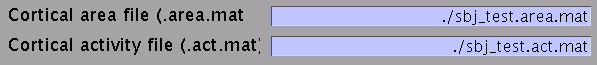
- Cortical activity file (.act.mat) consists of sets of some kind of activities (e.g., SPM t-value, cortical current at a time point) on the cortical surface model.
- Cortical area file (.area.mat) consists of sets of vertex indices representing a particular brain region (which can be the whole cortex) of the cortical surface model. For each vertex set, a string key is assigned, which is used to get the vertex set.
- M/EEG-MAT file (.meg.mat/.eeg.mat) has time-courses of M/EEG signals and extra channels.
- Head model file (.head.mat) has information about the structure of the subject's head. It is used to calculate the forward model by a numerical method (BEM).
- Leadfield file (.basis.mat) has leadfield matrix, which depends on the cortical surface model, head model, and M/EEG sensor position information included in the M/EEG-MAT file.
- Current variance file (.bayes.mat) has estimated current variance values and other model parameters of the hierarchical model of the M/EEG inverse problem.
- Cortical current file (.curr.mat) has estimated cortical currents.
Sample data
Sample data is available at http://vbmeg.atr.jp/?lang=en#DOWNLOAD
Unzipping this file creates a directory which including "vbmeg1.0_tutorial" directory. The data consist of
- MEG measurement (Yokogawa .ave file)
- fMRI analysis result (SPM voxel file)
of a passive viewing of a visual stimulus in the lower-right (LR) visual field (Yoshioka et al., 2008), and subject's
- MRI file ([.hdr/.img])
- cortical surface files (FreeSurfer)
- segmented gray matter file (SPM8)
The structure of the sample data is as follows:
- vbmeg1.0_tutorial/
- subjects/
- sbj_test/
- org/
- sbj_test.[hdr/img]
- FS4.2/ % FreeSurfer data
- SPM8/ % SPM8 data
- Yokogawa % Yokogawa MEG data
- org/
- sbj_test/
- subjects/
"subjects" directory is defined as the project root directory (see below). "sbj_test" directory includes all data for a subject.
Preparation of files required for VBMEG
MR image preprocessing (DICOM to ANALYZE, bias correction)
MRI data are required to create subject's cortical surface model. MRI data is often provided with DICOM format. However, VBMEG supports ANALYZE format. DICOM files can be converted to ANALYZE files with VBMEG function convert_dicom_nifti(dicom_file, output_dir). 'dicom_file' is a filename of an arbitrary DICOM file consisting MRI. Running this function, ANALYZE files (header and body of data) with prefix 'LAS_' are created (NIfTI files are also created with prefix 'RAS_').
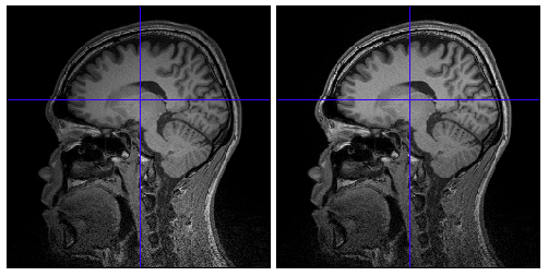
Because of inhomogeneous magnetic field, MR images are sometimes contaminated by low frequency variation of signal values, which causes on extraction of cortical surface from the images. VBMEG function vb_bias_correction_by_spm(analyze_file) can be used to correct signal values of MR images. Before executing this function, you need to set MATLAB path to SPM2/5/8 directory. After finished, bias corrected MRI files with prefix 'm' are created. The following figures are MR images before and after bias correction.
Cortical surface model
VBMEG can utilize cortex polygon models created with FreeSurfer or BrainVoyager. If you want to conduct inter-subject analysis, FreeSurfer is strongly recommended (see "Coregistration for inter-subject analysis"). BrainVoyager files can be used in VBMEG in their original format (.srf) while Freesurfer files have to be transformed within FreeSurfer. VBMEG assumes that the coordinate system of the poligon model coincides with the coordinate system of the MRI data. During preparation of the cortical surface model, the coordinate system is sometimes transformed into standard coordinates, so that structures other than the cerebral cortex (eg. cerebellum) can be discarded. In this case, the data has to be transformed back into their original coordinates before using them with VBMEG.
FreeSurfer
FreeSurfer automatically extracts the cortical surface model from the MRI data by the recon-all command. To use this command, an MRI file in MGZ format is required. ANALYZE format, which is widely used, can be converted to MGZ using the following FreeSurfer command:
mri_convert sbj_test.img 001.mgz
'001' denotes that it is the 'first' MR image. FreeSurfer can
construct the cortical surface model using two or more MR images (of the
same subject) by averaging them to increase S/N ratio of the MR image
from which the cortical surface model is extracted. In that case,
subsequent MGZ filename should be '002', '003', etc.
To create the FreeSurfer's subject directory, you can use mksubjdirs command as follows:
mksubjdirs $SUBJECTS_DIR/sbj_test
'sbj_test' is ID of the subject. All MGZ files have to be put in the $SUBJECTS_DIR/[sbj_id]/mri/orig/ directory as shown below:
cp 001.mgz (002.mgz 003.mgz ... if any) $SUBJECTS_DIR/sbj_test/mri/orig
The recon-all command processes MR image(s): (GM/WM boundary extraction, coregistration to the template, etc.) as in the following example:
recon-all -all -subjid sbj_test
It will take about 24 hours on a Linux PC with Xeon processor. After completion, surface files of the polygon model are saved in binary format. For VBMEG, the FreeSurfer data has to be saved in ASCII format. This can be done using the mris_convert command included with FreeSurfer. Executing the following commands in a Unix shell generates the files necessary for import of the cortical surface model into VBMEG:
cd [freesurfer_sbjdir]/sbj_test/surf/
mris_convert [lh/rh].smoothwm [lh/rh].smoothwm.asc
mris_convert [lh/rh].inflated [lh/rh].inflated.asc
mris_convert -c curv [lh/rh].smoothwm [lh/rh].curv.asc
mris_convert [lh/rh].sphere.reg [lh/rh].sphere.reg.asc
BrainVoyager
VBMEG can directly read BrainVoyager .srf files. However, since the coordinate system of the cortical surface model is Talairach by default in BrainVoyager a backward transformation of the coordinate system to be the original one is required.
fMRI data
- VBMEG function: vb_job_convert_spm (MATLAB console)
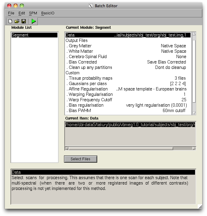
SPM2/5/8 generated t-values can be used to determine the relative amplitude of the prior current variance in the hierarchical Bayesian estimation. When the statistical parametric map appears on the display (vis SPM), the VBMEG function vb_job_convert_spm may be invoked to create a SPM-voxel file (.spm.mat), which can be imported into VBMEG. To do this, first add the VBMEG directory to MATLAB's path before running SPM. Next, run SPM to lunch its GUI, press "Result" button, choose the desired contrast and enter the appropriate parameters for determining probabilistic threshold. Then the following screen will appear:
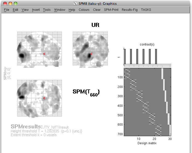
(note that in this figure the bottom half of the SPM results window is missing)
At this point, t-values and voxel coordinates are stored in the MATLAB workspace. Next, execute the VBMEG function vb_job_convert_spm on the MATLAB console in which SPM is running. You may be asked:
Normalized functional data?
To which you can can respond "yes" or "no". If you analyze the data on a template model, the voxel coordinate values in the template space must be converted to the original subject's space. For the backward transformation, the "_sn.mat" file is used. After that, enter the filename of the SPM-voxel file to which the SPM result is stored in a format readable by VBMEG.
Head model
You can use a spherical model to create the M/EEG forward model (leadfield). The spherical model is specified by the origin of the sphere and its radius. The MEG forward model with a spherical model is analytically calculated by the Sarvas equation which is not dependent on the radius of the sphere, while radii of spheres are also required for three-layers EEG forward model.
To obtain a more accurate forward model, VBMEG can create a cranial model from the subject's MRI. Required files for this calculation are:
- volumetric image of gray matter, created by using SPM8 "Segment" command (c1*.[hdr/img]).
- inner skull and outer skin surface files, created by FreeSurfer. To make these files, use mri_watershed command:
cd $SUBJECTS_DIR/sbj_test/mri
mri_watershed -surf bem_surf -useSRAS T1.mgz brain_bem.mgz
mris_convert lh.bem_surf_inner_skull_surface inner_skull_surface.asc
mris_convert lh.bem_surf_outer_skin_surface outer_skin_surface.asc
These files are specified in the "Create head model" GUI.
Setup and launch GUI
Installation
Execute the following commands in MATLAB in order to install the software:
> addpath(fullpath_to_vbmeg);
> vbmeg
--- Find VBMEG program directory
VBMEG program directory: /home/cbi/rhayashi/vbmeg
--- Set program directories to MATLAB path
--- Create global variable 'vbmeg_inst'
Here, the variable fullpath_to_vbmeg indicates the path of the top directory of the VBMEG software (“vbmeg”). If only the relative path is given, part of the GUI might not work properly. While the path settings will be preserved until MATLAB is closed, the command vbmeg has to be executed every time the memory is cleared, since this command defines a global variable ("vbmeg_inst").
Project manager startup
The project manager manages the execution of the various VBMEG GUIs and the parameters involved in each operation. It can be called after executing the vbmeg command by entering the following:
> project_mgr
The project manager GUI is shown.
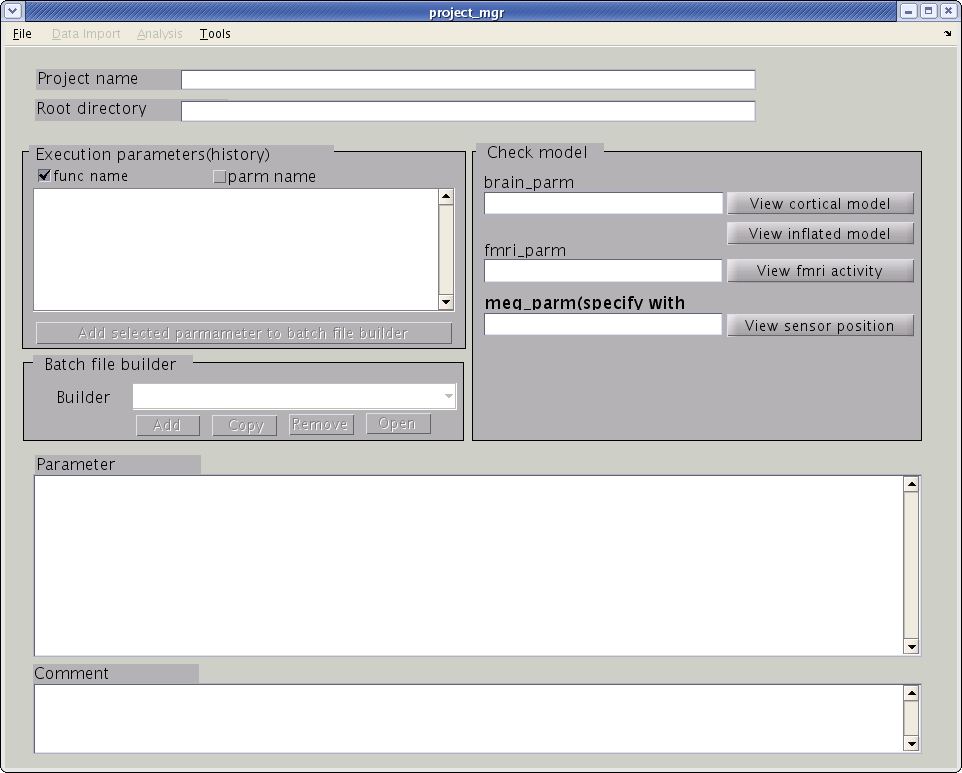
The next step is to specify a project file (.prj.mat), which is saved in the project root directory. This file contains jobs that are called by the project manager as well as the parameters for each job. All of the filenames created by VBMEG are specified as relative path from the project root directory.
- Creating a new project file
- From the project manager menu select [File]->[New project], then "Create new project" GUI will pop up.
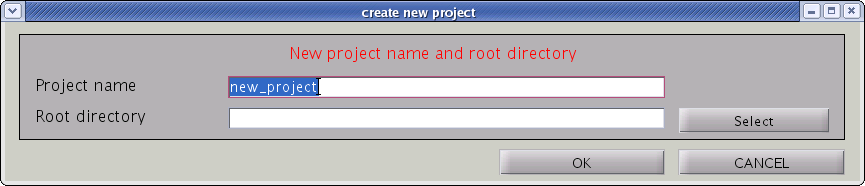
- Input “project_name” and ”project_root”, the directory in which the project should be saved. Press "OK" button.
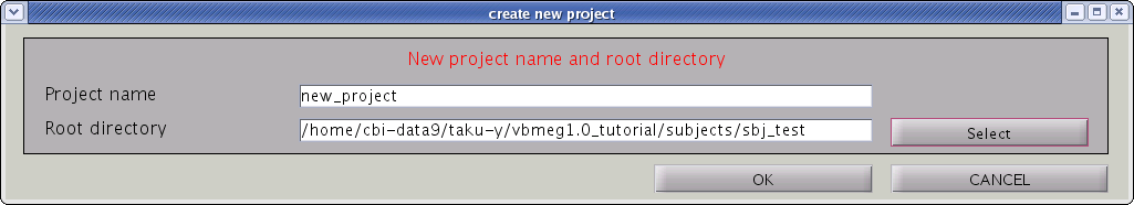
- Confirmation dialog will pop up. Press "OK" button.
- From the project manager menu select [File]->[New project], then "Create new project" GUI will pop up.
- Specifying an existing project file
- From the project manager menu select [File]->[Load project], then the file select dialog will pop up.
- Specify the project file.
- "project_name" and "project_root" will be appeared in their respective line of the project manager dialog.
Data import
This section gives how to import each of the files listed in the "VBMEG file format" section.
Cortical surface model
- VBMEG function: vb_job_brain
- From the project manager menu select [Data Import]->[Import
cortical model]. "Import cortical model" GUI will pop up. The default
cortical model is FreeSurfer. You can also import cortical surface
models of BrainVoyager.
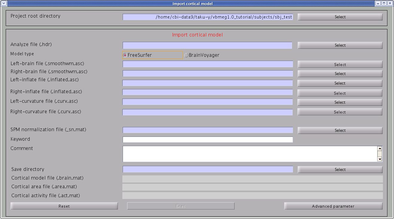
- Specify the files required.
- Specify ANALYZE (or NIfTI) header file of subject's MRI from which the cortical surface model was extracted (BrainVoyager or FreeSurfer).

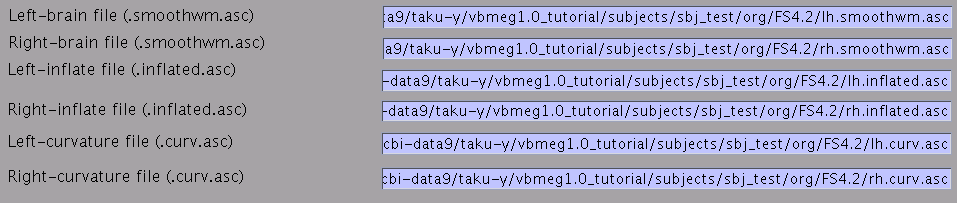
- Specify FreeSurfer files. Required files are smoothwm, inflated, curv for lh/rh.
- Specify SPM normalization file _sn.mat (optional). It is used to calculate the standard (template) brain coordinate values for vertices of the (individual) subject's cortical surface model.

- Specify the directory to which created files are saved.

- Filenames are automatically set using MRI filename.

- Press “Exec” button to start import of the cortical model.
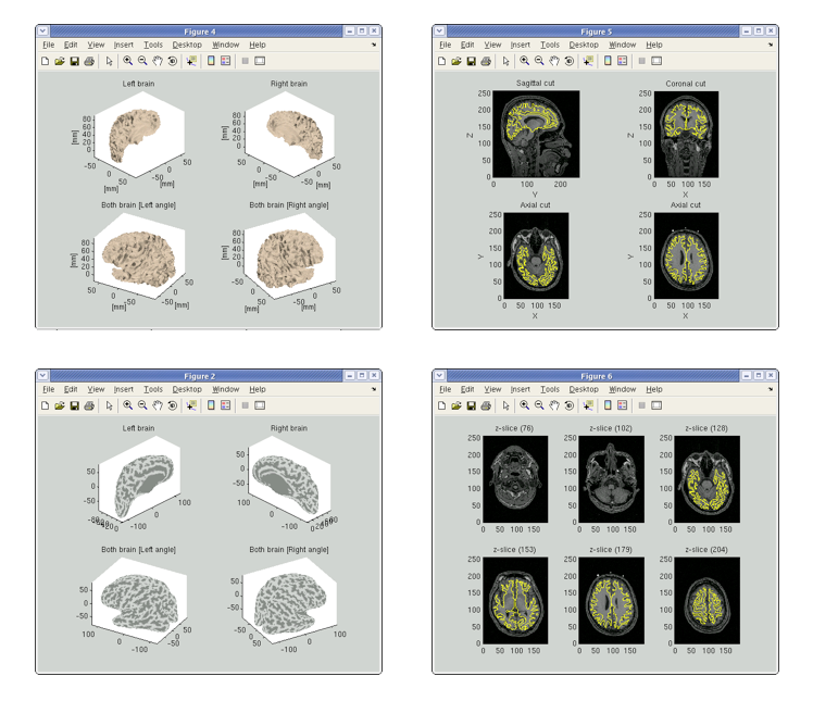
After processing three files will be created: the cortical surface model file (.brain.mat), cortical activity file (.act.mat) and cortical area file (.area.mat). The following figures will be shown. Check if the cortical surface model (yellow line) is aligned with the gray/white matter boundary in MR image.
If you specified the SPM normalization file (_sn.mat) in the GUI, the standard brain coordinate values of the Talairach and MNI305 templates are appended to the cortical surface model file. In addition, VBMEG creates 3 files: _brodmann.area.mat, _aal.area.mat, and _atlas.act.mat, which include anatomical label data on the cortical surface model.
MEG data
- VBMEG function: vb_job_meg
VBMEG can import MEG data measured by a Yokogawa system (MegLaboratory; .raw, .ave, .con). The MEG sensor position should be transformed into SPM-Analyze (RAS, origin at the center of MRI volume) coordinate system. The coregistration methods supported by VBMEG are the standard method offered by MegLabotory (determination of the marker location by means of MRI) and the method developed by Shimadzu and ATR (three dimensional matching of the face; Kajihara et al., 2004). To import MEG data, follow the below steps:
- Select [Data Import]->[Import MEG data]->[Yokogawa] from the
project manager menu. "Import YOKOGAWA MEG data" GUI will pop up.
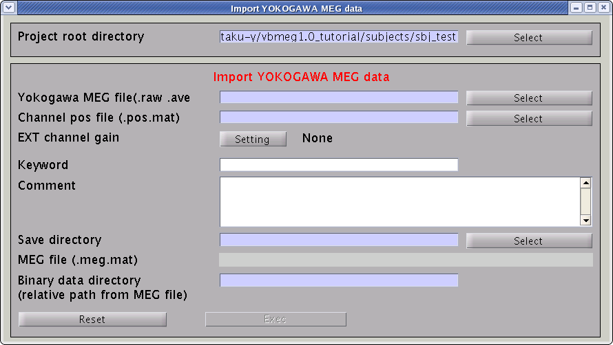
- Specify the required MEG data files.
- Specify Yokogawa MEG file (.raw, .ave, .con).

- Specify positioning file (.pos.mat). This is used to transform sensor coordinate values.

- Specify the directory to which created file will be saved.

- The MEG-MAT file name is automatically set. In addition, the directory, in which the MEG time course is saved, is also created.

- Press “Exec” button to start import.
The data, now formatted for VBMEG, are saved in a MEG-MAT file.
To check signals of MEG data, you can M/EEG viewer. Select [Tools]->[View MEG/EEG data] from the project manager menu. Then "View MEG/EEG data" dialog will pop up.
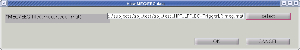
Select MEG-MAT file and press "OK" button. MEG/EEG viewer GUI will pop up.
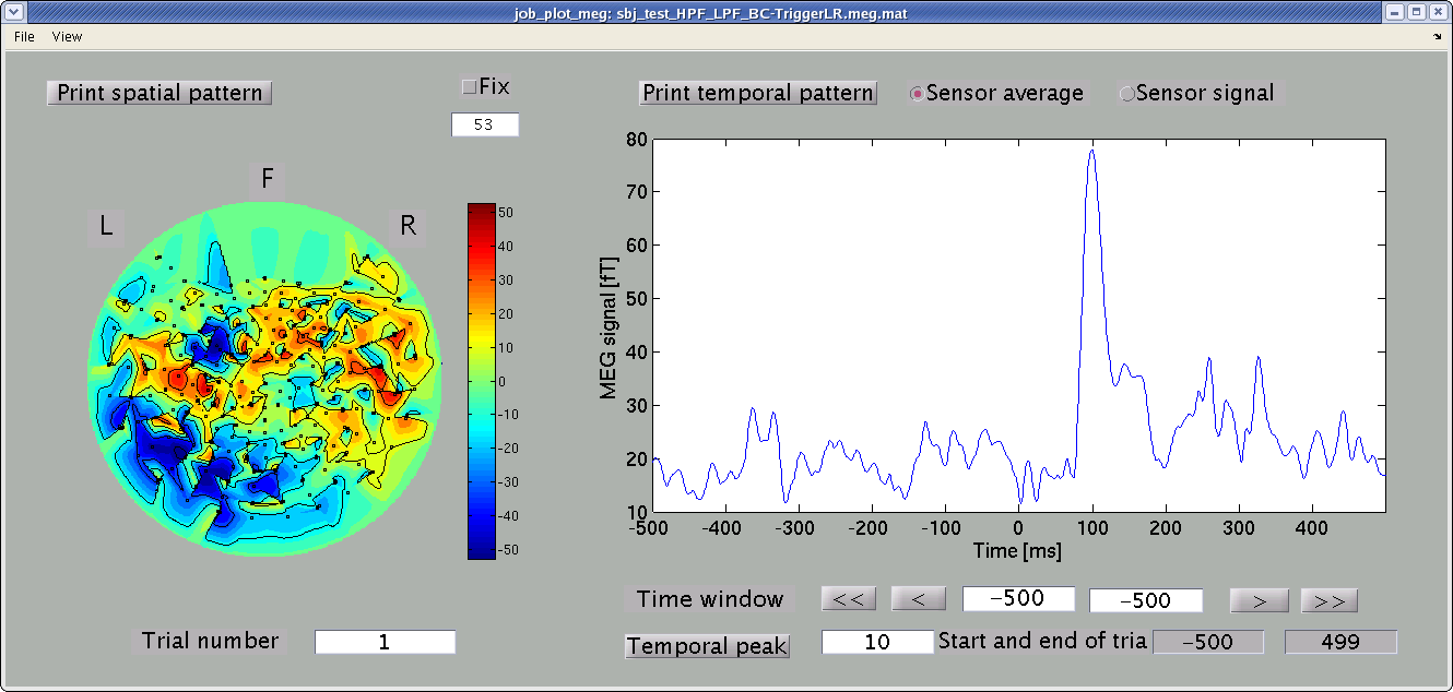
Spatial map and time course of MEG signals are shown in the left and right panel. You can select arbitrary time window, from which the spatial map is obtained, by dragging the cursor on the right panel.
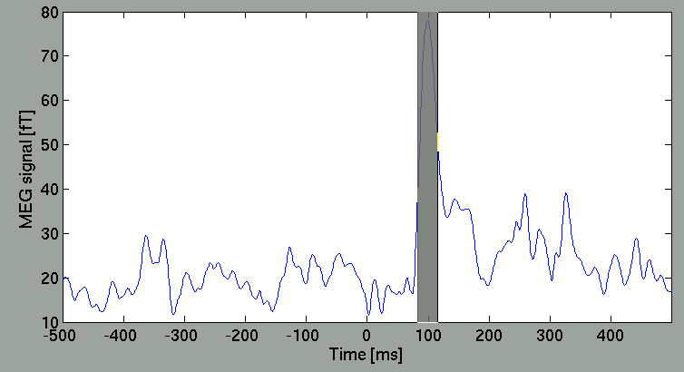
Then, the spatial map will be updated.
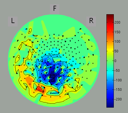
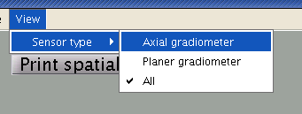
The spatial map may be discontinuous because of the configuration of the direction of sensors of some MEG systems is arbitrary (as of MEG system in ATR). You can select axial sensors to be plotted from the menu of GUI.
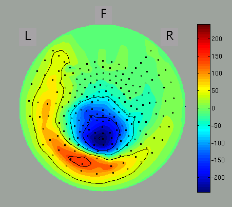
If the direction of axial sensors is continuous spatially, the spatial map of MEG signals is smooth as in the figure.
EEG data
- VBMEG function: vb_job_meg
Data obtained by a Biosemi EEG system (.bdf) can also be imported. Screening of the individual session and trial data for artifacts is recommended before import, but can also be conducted after import into VBMEG. The EEG sensor position has to be transformed into SPM-Analyze (RAS, origin at the center of MRI volume) coordinate system before import. The coregistration method supported by VBMEG is the one developed by Shimadzu and ATR (three dimensional matching of the face; Kazihara et al., 2004). EEG data can be imported by following the steps below:
- Select [Data Import]->[Import EEG data]->[Biosemi] from the
project manager menu. "Import Biosemi EEG data" GUI will pop up.
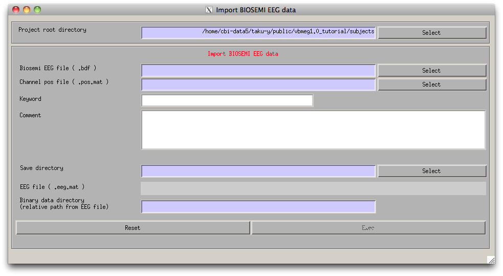
- Specify the required EEG data files.
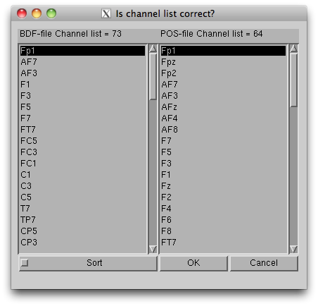
- Press “Exec” button to start the import, then the channel lists,
included in the BDF file and the POS-MAT file, are shown. The order of
channels does not matter, but you should check if all the EEG channels
(on the scalp) in the BDF file are included in the POS-MAT file. Some
extra channel (EOG, EMG, trigger recording) can be included in the BDF
file, so the lengths of the lists can also be different. Pressing "Sort"
button sorts the order of display and does not affect to import
process.
- The data, now formatted for VBMEG, are save in an EEG file (.eeg.mat).
fMRI data
- VBMEG function: vb_job_fmri
SPM-Voxel file (.spm.mat) can be imported by following the steps below:
- Select [Data Import]->[Import SPM data] from the project manager menu. "Import SPM voxel data" GUI will pop up.
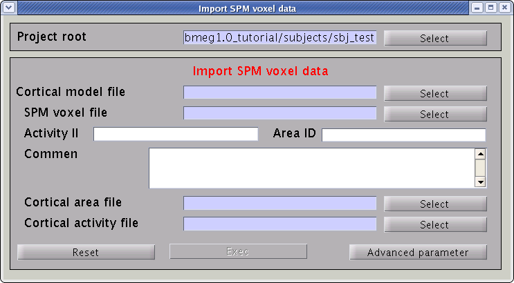
- Specify the required files.
- Specify the cortical surface model file (.brain.mat), onto which voxels are projected.

- Specify the SPM-Voxel file, which includes voxels of SPM t-values.

- Specify IDs of activity map and cortical area.

- Specify the cortical activity file and cortical area file. The
activity map and cortical area are stored in these files with specified
IDs.
- Specify the cortical surface model file (.brain.mat), onto which voxels are projected.
- Press “Exec” button to start the data import.
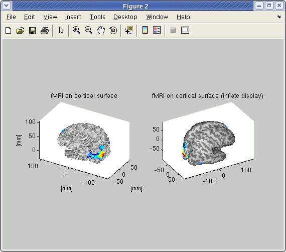
The t-values provided by the SPM-Voxel file are mapped onto the cortex vertices and regirstered in the cortical activity file with the identifier you specified. Additionally, voxles with a t-value exceeding the threshold will be registered an individual area of the cortex and as such saved in the cortical area file. The following figure shows the result of the import of the "LR" result of SPM8.
Head model
- VBMEG function: vb_job_head_3shell
You can make a realistic head model to improve accuracy of the leadfield calculation by following the steps below:
- Select [Data Import]->[Import head
model]->[SPM/FreeSurfer/Curry v4.5] from the project manager menu.
"Create head model" GUI will pop up.
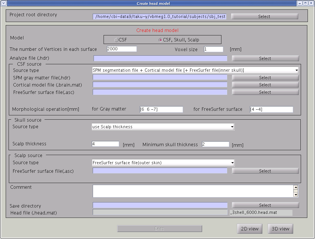
- Specify files and parameters.
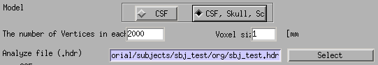
- Specify head model type. For MEG check "CSF", making a head model consisting of single layer (celebro-spinal fluid; CSF). Then the number of vertices of the CSF layer are automatically set (6,000 by default). The Analyze/NIfTI image is also required.

- For EEG, check "CSF, Skull, Skalp", which will make a head model consisting of three layers (CSF, Skull, Scalp). The number of vertices for each of the three layers is 2,000.
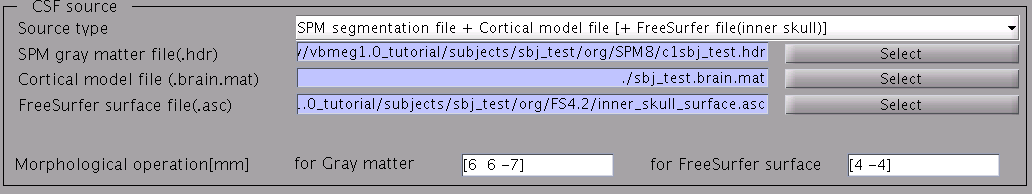
- Specify files and parameters for creating the CSF surface. Required files are the SPM8 gray matter file (c1*.hdr), VBMEG cortical surface model file, and FreeSurfer inner skull surface file (see section "Head model" of "Preparation of files required for VBMEG").
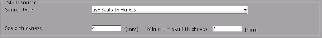
- Specify parameters for creating the skull surface. You can use the default parameters.
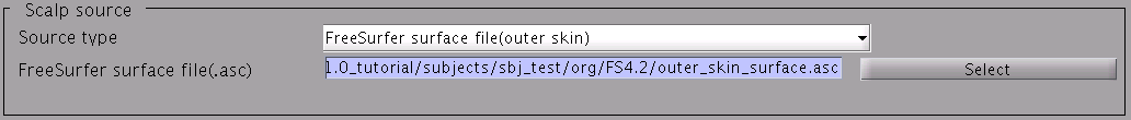
- Specify files and parameters for creating the scalp surface. The required files is FreeSurfer outer skin surface file (see section "Head model" of "Preparation of files required for VBMEG").
- Specify the directory to which the head model file is saved.

- Press "Exec" button to start making the head model.
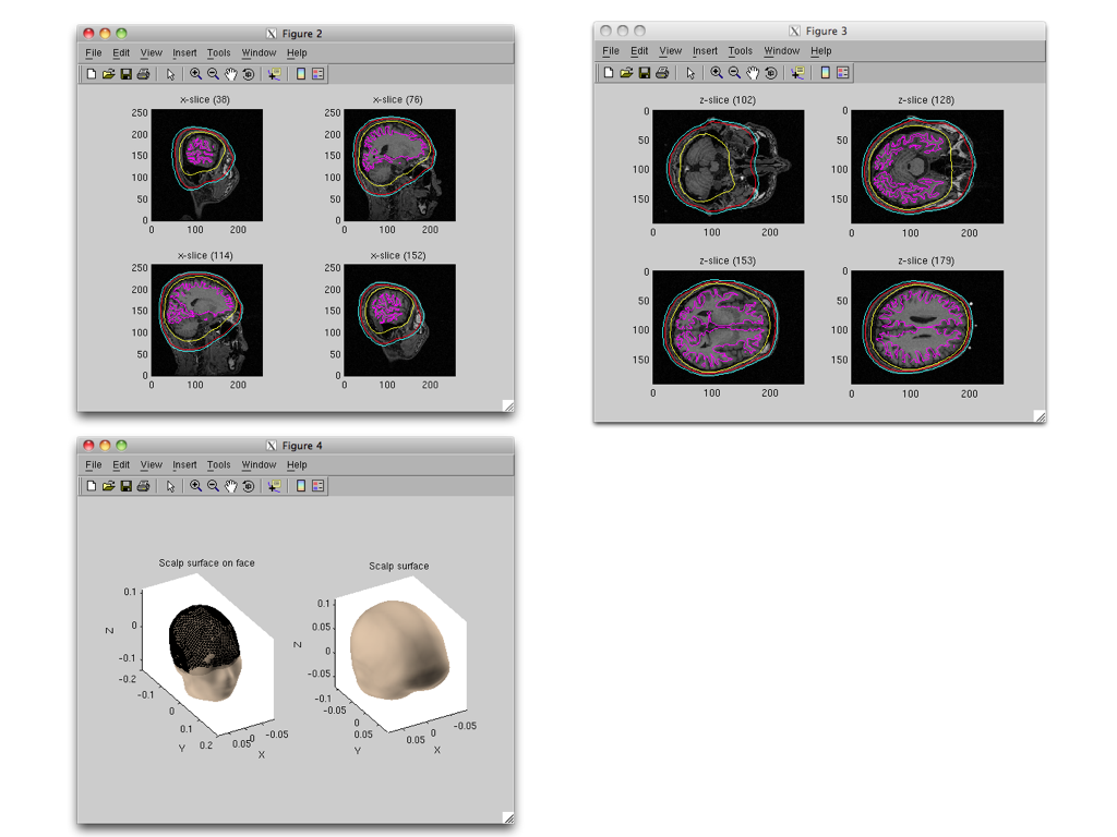
A head model file will be created and figures as below will be appeared. In this example there is a CSF single layer (yellow line) model for MEG. Check if the CSF surface correctly aligned with the MR image.
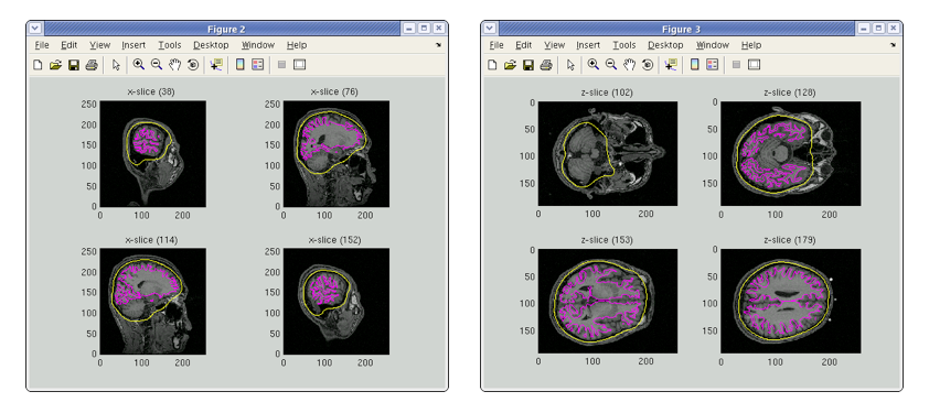
Specifying a three layer model for EEG gives the following figures, consisting of CSF (yellow), skull (red), and scalp (light blue) surfaces. In the last figure, the scalp surface is superimposed on the face model.
Cortical current estimation
The estimation of the electric current source with VBMEG is done in three steps: Leadfield calculation, current variance estimation and finally, current timecourse estimation.
Leadfield calculation
- VBMEG function: vb_job_leadfield
Leadfield can be calculated by following the steps below:
- Select [Analysis]->[Calculate leadfield] from the project manager menu. The "Leadfield calculation" GUI will pop up.
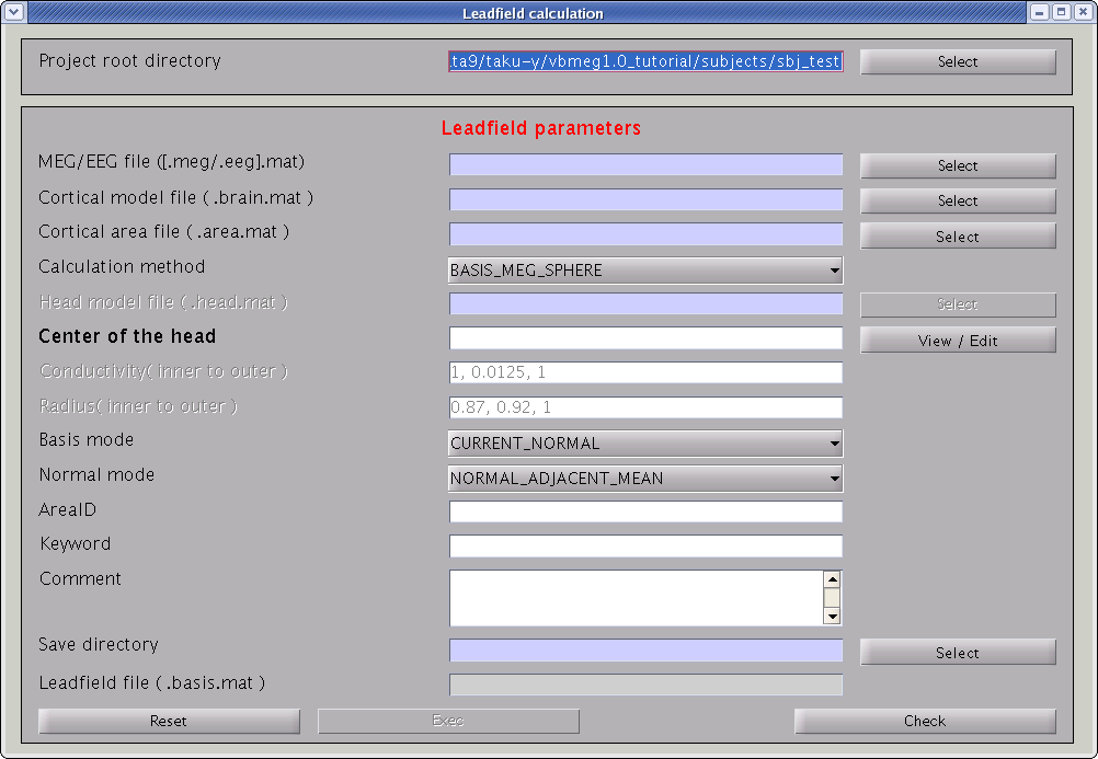
- Specify the required files and parameters.
- Specify the M/EEG-MAT file and cortical model file. You do not
need to specify the cortical area file (the field is not necessary and
will be removed in a future version).
- Specify the method for leadfield calculation. "BASIS_MEG_BEM" is the option to use BEM for calculation of the leadfield.

- The head model file must be specified for BEM.

- Do not modify parameters here. These parameters are used for advanced users.

- Specify the directory to which the leadfield file is saved. The filename is automatically set using the MEG-MAT filename.

- Specify the M/EEG-MAT file and cortical model file. You do not
need to specify the cortical area file (the field is not necessary and
will be removed in a future version).
- Press “Exec" button to start the leadfield calculation.
- The result is saved in the leadfield file (.basis.mat).
The leadfield at M/EEG sensors are calculated for every vertex of the cortical surface model.
Current variance estimation
- VBMEG function: vb_job_vb
The hierarchical Bayesian method for estimation of brain activity estimates variance of the electric current from the MEG data. Once the current variance is obtained, we can calculate the linear inverse filter, which will yield the electric current estimation when multiplied with the MEG data matrix. Here, we explain how to arrive at the electric current variance using VBMEG. From the project manager menu, choose [Analysis]->[Estimate current variance] to open the "Current variance estimation" GUI. This GUI displays a variety of parameters, which have to be chosen carefully. The following provides information on how to choose the parameters and gives examples.
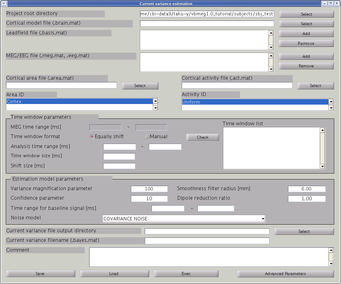
Input files
First, the cortical model file, leadfield file and MEG-MAT file have to be specified. To select leadfield file and MEG file, press the “Add” button. VBMEG can estimate the current distribution for multiple sessions at the same time. The below figure displays an example with a single session.
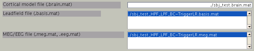
You can specify multiple leadfield/MEG-MAT files across sessions. The leadfield file and MEG-MAT file must correspond with each other: the first leadfield file is calculated from the first MEG-MAT file. The same holds for the second, third ones.
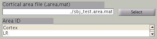
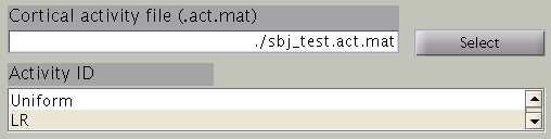
Cortical area and activity
In the next step, cortical area and cortical activity is selected. The cortical area information is used to specify the areas in which dipoles are assumed. The cortical activity information is used to determine the hyper parameters. In case you are importing fMRI data with VBMEG, it is recommended to label the cortical areas and the related activity according the conducted MEG study. The standard cortical area ("Cortex") and cortical activity ("Uniform") are registered without fMRI data.
The cortical area ID ”Cortex” includes all vertices of the cortical model; when ”Cortex” is selected dipoles are assumed at all vertices of the cortex. The cortical activity ID ”Uniform” assumes that the whole cortex activation follows a uniform pattern. If no fMRI data is given, the cortical area ID “Cortex” will be used for the estimation with the cortical activity ID “Uniform”. Here we have imported fMRI data, so cortical activity ("LR") is used to determine hyper parameters.
Time window parameters
VBMEG divides the MEG data into time windows of suitable length and estimates the current distribution separately for each of these windows. Based on the MEG-MAT file specified, the dafault parameters in the ”Time window parameters” sections will automatically be set to the default values. In the default setting, a single time window covers the whole time series. That is to say, the prior distribution of the electric current is assumed to be the same at each time point.
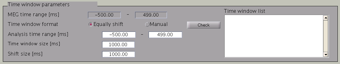
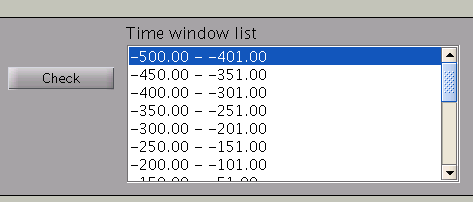
Time windows separation is favorable in case the cortical activity changes in location with time (Shibata et al., 2008, Callan et al., 2010). To divide the time window, two options are available: you can either set time window width and window shift (equally shift) or manually set every time window (manual). The two options can be selected with the ”Time window format” check box. In case of multiple time windows, window width and time shift have to be set accordingly. In our example, the MEG data was divided into 100 ms time windows. The ”Shift size” is set to 50 ms, i.e. the windows overlap 50 ms. In the overlapping regions, the electric current distribution is estimated independently. However, the electric current itself will be estimated as the average over the estimations for each window.
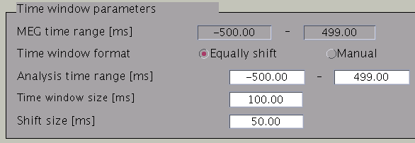
Pressing the ”Check” button returns a list of the individual time windows.
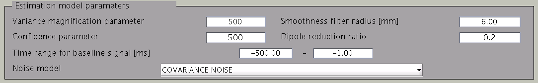
Estimation parameters
The figure below shows how the estimation parameters in the GUI should be set.
VBMEG has the following estimation parameters:
- Smoothness filter radius: VBMEG makes use of a smoothing filter that can be described by exp(-(d/R)^2), where d is the distance between two vertices measured along the cortical surface and R is the “Smoothness filter radius”. The standard value for R is 6mm.
- Dipole reduction ratio: In case the number of vertices in the cortical model should be too high, it can be reduced by setting the value for ”Dipole reduction ratio”, e.g. for a cortical model with 20,000 vertices, setting the Area ID to ”Cortex” and ”Dipole reduction ratio” to 0.2, will reduce the number of dipoles left over to 4,000.
- Noise model parameters: The standard for the ”Noise estimation model” is ”COVARIANCE NOISE”. The time interval set in ”Time range for baseline signal” determines which part of the MEG data. VBMEG uses to estimate 1) the covariance matrix of the observation noise and 2) the baseline current variance. Usually, this time interval is set as the baseline interval (time before trigger onset).
- Hyper parameters: In the hierarchical Bayesian estimation, two hyper parameters control the electric current estimation, the “Variance magnification parameter” (in the following refered to as m0) which controls the current strength and the ”Confidence parameter” (in the following gamma0), a coefficient of confidence in the fMRI data. The higher the value of m0, the higher the power of the electric current is estimated. In standard cases a value of m0 = 100 is recommended. If extremely high electric currents are expected, such as in visual color grading experiments, m0 can be set as high as 500. If fMRI data is available, the standard value for the confidence parameter gamma0=100. If no fMRI data is available or the conditions for fMRI and MEG experiment differ significantly set gamma0=10. Conversly, if the experiments for fMRI and MEG are equal, the value can be set as high as gamma0=500. A high value of gamma0 (e.g., 100000) results in the Wiener filter estimation (Kajihara et al., 2004).
Output file
Finally, select the ”Current variance file directory” and the ”Current variance filename”, where the results will be stored. Note that "Current variance file" does not include current time course, but consists of current variances and other model parameters, from which the inverse filters are calculated.

After having set the parameters, press the ”Exec” button to start the estimation.
Current timecourse estimation
- VBMEG function: vb_job_current
Cortical current time course can be calculated by multiplying the inverse filters, obtained using the estimated current variance and other model parameters. This calculation can be performed by following the steps below:
- From the project manager menu, select [Analysis]->[Estimate current]. The "Current estimation" GUI will pop up.
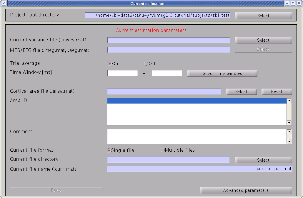
- Specify the files and parameters required.
- Specify current variance file (.bayes.mat). GUI will automatically
put M/EEG-MAT file (.meg.mat/.eeg.mat) from which current variance was
estimated. You can overwrite this parameter.

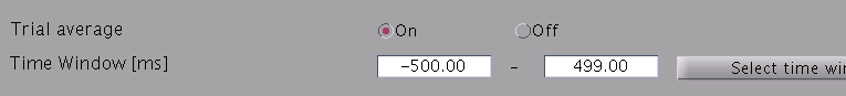
- Specify estimation parameters. If "Trial average" is "On", current
timecourses are calculated for MEG data averaged across trials. You
also can set a time window sorter than one used in the "Current variance
estimation". By default, the time window covering whole data is used.
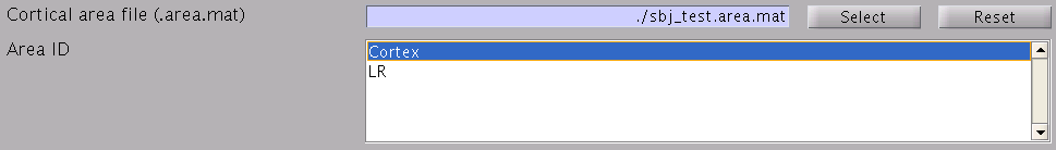
- Specify cortical area on which current time courses are
calculated. If the size of the MEG data is too large (many trials, long
time window), this option is preferable to reduce the size of current
timecourses.
- Specify how to store the body of current timecourse data. If the
"Single file" option is selected, estimated current time courses for all
trials are saved into a single file, while if the "Multiple files"
option is selected, current time courses are saved into different files
for each trial.

- Specify the directory to which the cortical current file is saved.
The filename is automatically set using current variance filename.

- Specify current variance file (.bayes.mat). GUI will automatically
put M/EEG-MAT file (.meg.mat/.eeg.mat) from which current variance was
estimated. You can overwrite this parameter.
- Press "Exec" button to start estimation of cortical current time course.
The estimated current timecourse is then saved into a cortical current file (.curr.mat).
View cortical current
- VBMEG function: job_plot_currentmap
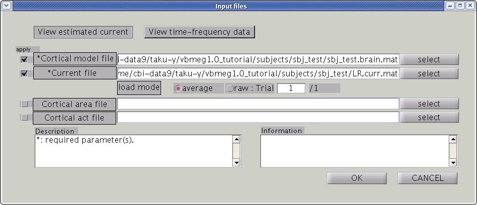
To look at the estimated cortical current, select [Tools]->[View
estimated current] from the project manager menu. Then file select
dialog will pop up. You need to specify the cortical current file and
the cortical model file. The cortical currents will be mapped on the
cortical surface model. You can also specify cortical area and activity
map files.
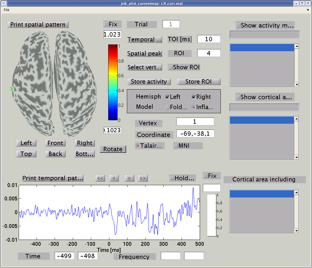
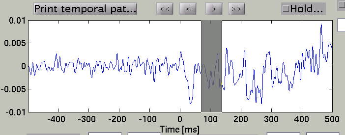
GUI of the cortical current viewer will pop up. In the left, the
selected cortical surface model is plotted. The time course on the
bottom is the estimated current of the selected vertex. Just after
launch the GUI, the 1st vertex is selected ("Vertex index" edit box).
The selected vertex is marked by a green cross (left hemisphere in the
figure).
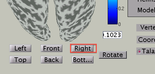
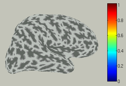
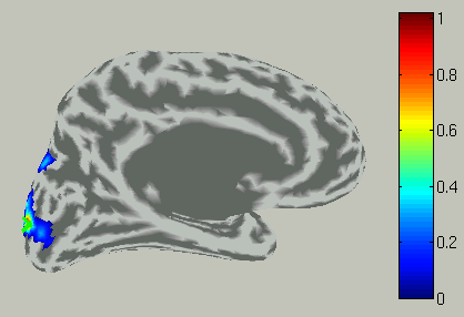
Push "Right" button to change the viewpoint to look at the cortical surface model from right.
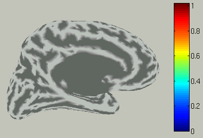
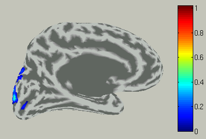
You can choose which hemisphere is shown. To suppress the right hemisphere plot, uncheck the "Right" check box.
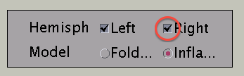
The the right hemisphere will disappear and the left hemisphere is shown in the medial view.
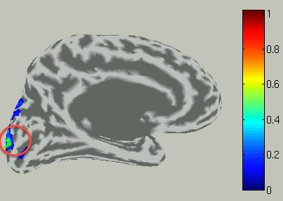
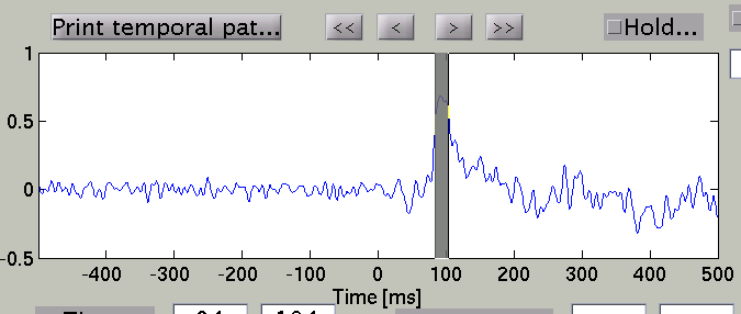
In the time course plot, you can specify an arbitrary time window. Here
the latency of visual evoked field (around 100ms) is chosen.
Accordingly, the spatial pattern of the cortical current is shown with averaging across the time window.
To choose a vertex (current dipole), push "Select vertex" button and click a point of the cortical surface model.

Then the green cross moves to the point specified,
and the time course plot is changed to the one on the selected vertex.
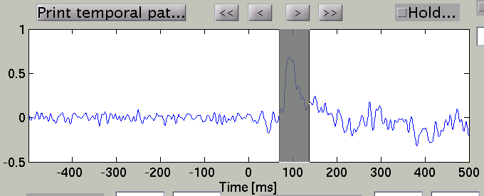
By pressing "Temporal peak" button, you can find the peak of the timecourse within the time window.
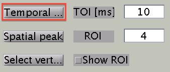
The width of the time window after the temporal peak search is in the "TOI" editbox.
The spatial pattern of the cortical current is also updated reflecting the update of the time window.
Advanced topics
Coregistration for inter-subject analysis
- VBMEG function: vb_job_add_sphcoord, vb_job_coreg_brain
To conduct inter-subject analysis, a coregistration matrix to a template cortical surface model is required for each subject's cortical surface model. A template cortical surface model "fsaverage" from FreeSurfer (see FreeSurfer's web site for more detail about this data) is attached with VBMEG software. An activity map (e.g., cortical current at a timepoint) of the cortical surface model of an individual subject (referred to as "source"), J_s, is transferred to the one on another cortical surface model (referred to as "target", usually a template brain), J_t, by multiplying the coregistration matrix C: J_t=C*J_s.. Each component of the projection matrix, C_{ij}, is proportional to exp(-(d_{ij}/R)^{2}), where R is a tunable coefficient and d_{ij} is the distance between the i-th vertex of the template model and the j-th vertex of the source model, on a common coordinate system (3D volume coordinate and 2D cortical surface coordinate supported by VBMEG). Intuitively, the coregistration matrix represents closeness of the vertices of the template and source models.
The calculation of the coregistration matrix for each subject's model consists of 2 steps:
- (optional, but strongly recommended) import coordinate values commonly used in the template model (vb_job_add_sph_coord).
- calculate the coregistration matrix using the coordinate values (vb_job_coreg_brain).
If you used FreeSurfer, spherical coordinate values are assigned to each vertex. These are calculated such that sulci and gyri of the subject's cortex align to the ones of "fsaverage" model and saved to "[lh/rh].sphere.reg(.asc)". To import them into the cortical surface model file, vb_job_add_sphcoord is used. The following is an example:
>> proj_root = './subjects/';
>> brain_parm.brain_file = 'sbj_test/sbj_test.brain.mat';
>> brain_parm.brain_sphL = 'subjects/sbj_test/org/FS4.2/lh.sphere.reg.asc';
>> brain_parm.brain_sphR = 'subjects/sbj_test/org/FS4.2/rh.sphere.reg.asc';
>> brain_parm.key = 'sphere.reg'; % arbitrary string available
>> vb_job_brain_add_sphcoord(proj_root,brain_parm);
The spherical coordinate values are then added to the cortical
surface model file. Note that "brain_file" specifies a relative path
from the project root directory ("proj_root"), while "brain_sph[L/R]"
specifies the source file directly. "demo/vb_test_gave2.m" in "demo"
directory is a sample script.
A coregistration matrix is calculated by using vb_job_coreg_brain. Before running this function, you should copy the "fsaverage" model to subject's directory:
mkdir your_work_dir/vbmeg1.0_tutorial/subjects/fsaverage
cp your_vbmeg_dir/functions/tool_box/freesurfer4.5/* your_work_dir/vbmeg1.0_tutorial/subjects/fsaverage
Then run vb_job_coreg_brain as below:
>> coreg_parm.source_file = './subjects/sbj_test/sbj_test.brain.mat';
>> coreg_parm.source_key = 'sphere.reg';
>> coreg_parm.target_file = './subjects/fsaverage/fsaverage.brain.mat';
>> coreg_parm.target_key = 'sphere.reg'; % prospectively registered to fsaverage.brain.mat
>> coreg_parm.key = 'fsaverage.sphere.reg';
>> vb_job_coreg_brain(coreg_parm);
The coregistration matrix is added to "sbj_test.brain.mat".
Grandaverage
- VBMEG function: vb_job_grandaverage
The grand average of cortical current across trials and subjects is calculated by vb_job_grandaverage. In the above example we only have the cortical current timecourse of a single subject. An example of the calculation of cortical current timecourse on the template brain (fsaverage.brain.mat) is shown below:
>> avr_parm.curr_file = {'./subjects/sbj_test/LR.curr.mat'};
>> avr_parm.brain_file = {'./subjects/sbj_test/sbj_test.brain.mat'};
>> avr_parm.key = {'fsaverage.sphere.reg'};
>> avr_parm.tbrain_file = './subjects/fsaverage/fsaverage.brain.mat';
>> avr_parm.curr_file_out = './subjects/fsaverage/LR.curr.mat';
>> vb_job_grandaverage(avr_parm);
Artifact rejection with extra-dipole
M/EEG signals are sensitive to eye movement artifacts. VBMEG support the extra-dipole method, which models eyeball artifact sources by current dipoles and estimates their current simultaneously the cortical current (Fujiwara et al., 2009; Morishige et al., 2009). It has been shown that eye movement artifacts are successfully removed while not affecting the estimation of the cortical current correlated with the eye movements (Fujiwara et al., 2009). In addition, cardiac artifacts are also removed (Morishige et al., 2009). To use the extra-dipole method, follow the steps below:
- Create extra-dipole position file (.mps.mat) using the GUI to place the extra-dipoles on the eyes.
- Calculate the leadfield for the extra-dipoles.
- Estimate current variance on the MATLAB console (the extra-dipole method not supported on "Current variance estimation" GUI).
Create extra-dipole position file (.mps.mat)
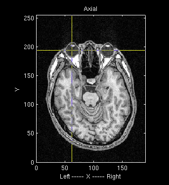
- Run the VBMEG command vb_mri_point_select on the MATLAB console and choose the subject's MR image. Then "MRI point select" GUI will pop up.
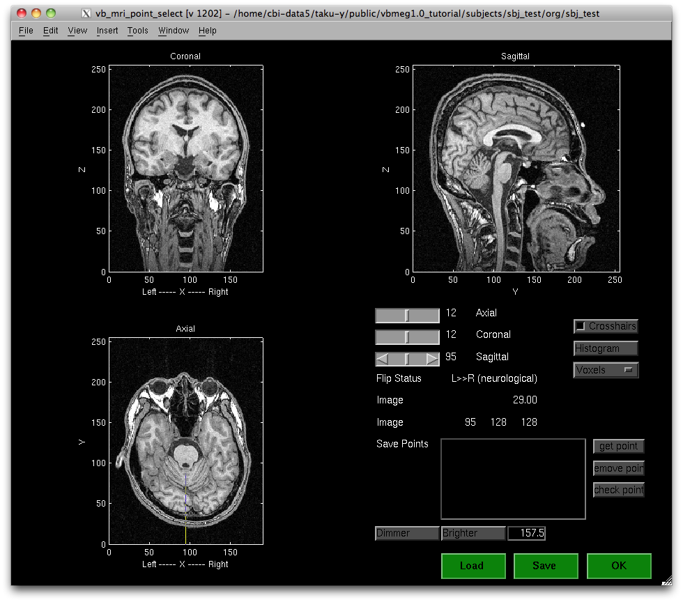
- Choose the left eyeball position on the MR image.
- Press the "get point" button then the "Enter the point name" dialog will pop up. Choose "Left eye".
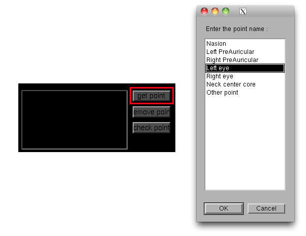
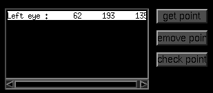
- "Left eye" is added to "Save points" list.
- Choose the right eyeball the same way.
- Press "Save" button to save the coordinate values of the selected points.
Manually create .mps.mat file
If you want to place extra-dipoles at places other than eye balls, you should use the following MATLAB code.
% directories and files
work_dir  = '/home/cbi-data9/taku-y/public/extdip/';
sbj_dir   = [work_dir 'subjects/sbj_test/'];
proj_root = sbj_dir;

% put extra-dipoles
Pointlist = cell(3,1);

% --- left eye
Pointlist{1}.coord_type = 'SPM_Right_m';
Pointlist{1}.name       = 'Left eye';
Pointlist{1}.point      = 1e-3*[-33.5 64 0];

% --- right eye
Pointlist{2}.coord_type = 'SPM_Right_m';
Pointlist{2}.name       = 'Right eye';
Pointlist{2}.point      = 1e-3*[28.5 65 0];

% --- heart
Pointlist{3}.coord_type = 'SPM_Right_m';
Pointlist{3}.name       = 'Heart';
Pointlist{3}.point      = 1e-3*[0 0 -300];

% make .mps.mat file
save([sbj_dir 'brain/sbj_test.mps.mat'],'Pointlist');
Here 30cm below (1e-3*[0 0 -300])the center of MR image, which is the origin of the coordinate system used in VBMEG ('SPM_Right_m'), is tentatively defined as a place from which cardiac artifacts come. In this code, extra-dipoles are assumed at three places and nine dipoles for x, y, z directions at each place. You can add four or more extra-dipoles by modifying the code.
Calculate leadfield for extra-dipoles
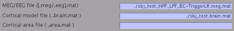
To calculate the leadfield for the extra-dipoles, you need to run vb_job_leadfield_extra from the MATLAB console. The following is an example (note that "meg_file", "mps_file" and "basis_file" are relative path from proj_root):
>> proj_root = './subjects/';
>> extra_basis_parm.meg_file = 'sbj_test/sbj_test_HPF_LPF_BC-TriggerLR.meg.mat'; % MEG file including sensor position of the session to be analyzed
>> extra_basis_parm.mps_file = 'sbj_test/sbj_test.mps.mat'; % Extra-dipole position file you created
>> extra_basis_parm.basis_file = 'sbj_test/sbj_test_HPF_LPF_BC-TriggerLR_eyes.basis.mat'; % arbitrary filename to which the leadfield matrix of the extra-dipoles will be stored.
>> vb_job_leadfield_extra(proj_root,extra_basis_parm);
After finished, the leadfield file for the extra-dipoles are created.
Check leadfield of extra-dipole
Before conducting estimation, you should make sure that the spatial pattern of the extra-dipole matches with the spatial pattern of the artifact you want to remove. The following code plot the leadfield of the 7-th component of the extra-dipole created with the MATLAB code in "Manually create .mps.mat file", corresponding to x-direction placed at the heart:
% directories and files
work_dir   = '/home/cbi-data9/taku-y/public/extdip/';
sbj_dir    = [work_dir 'subjects/sbj_test/'];
meg_file   = [sbj_dir 'meg/sbj_test_UR.meg.mat'];
basis_file = [sbj_dir 'basis/sbj_test_extdip.basis.mat'];

% get MEGinfo (sensor type depends on the system you use)
MEGinfo = vb_load_meg_info(meg_file,5);
ix1     = find(MEGinfo.ChannelInfo.Type==2); % axial sensor
ix2     = find(MEGinfo.ChannelInfo.Type==3); % planar sensor

% get sensor position
pick = vb_load_sensor(meg_file);
pick = pick(1:(size(pick,1)/2),1:3);

% load leadfield
load(basis_file,'basis');

% plot leadfield
pick1 = pick(ix1,:); % axial sensor
pick2 = pick(ix2,:); % planar sensor

% --- heart (x)
clim_val = 1e-6*[-0.1 0.1];
figure('Name','Heart (x)');
subplot(2,1,1);
vb_plot_sensor_2d(pick1,basis(7,ix1),clim_val);
axis equal off;
colorbar;
subplot(2,1,2);
vb_plot_sensor_2d(pick2,basis(7,ix2),clim_val);
axis equal off;
colorbar;
The following figure will appear:
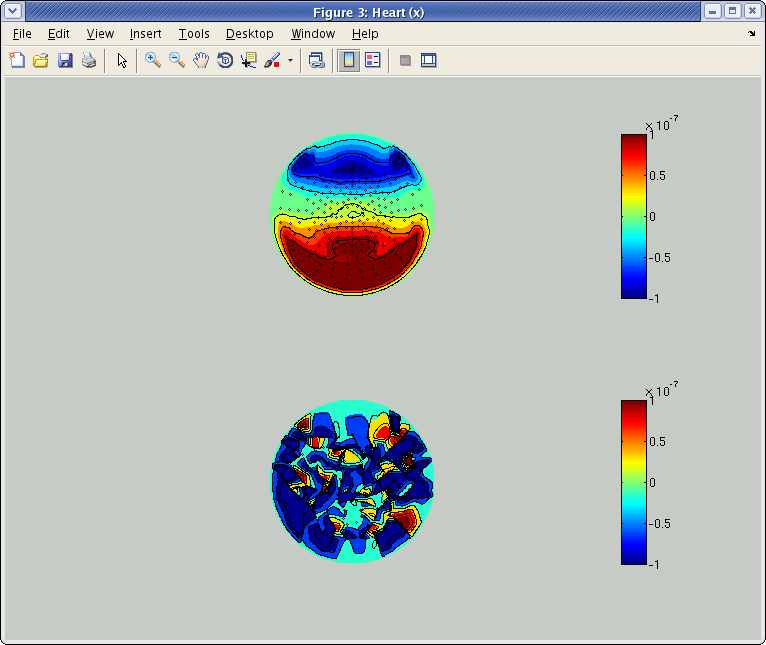
The above and below show spatial patterns of the leadfield at axial and planar sensors, respectively, of Yokogawa 400ch system in ATR. The actual figure you will see depends on the sensor configuration of your system.
Estimate current variance on MATLAB console
To estimate current variance, you need to manually set the parameters for extra-dipoles in bayes_parm.extra:
>> proj_root = './subjects/';
>> ...
>> bayes_parm.extra.basisfile = 'sbj_test/sbj_test_HPF_LPF_BC-TriggerLR_eyes.basis.mat'; % Multiple sessions not supported yet
>> bayes_parm.extra.extra.a0 = (5e-9)^2*ones(6,1);
>> bayes_parm.extra.Ta0 = 100*ones(6,1);
>> bayes_parm.extra.a0_physical = true;
>> ...
>> vb_job_vb(proj_root,bayes_parm);
The following two issues should be noted:
- Number of extra-dipoles: we have specified 2 position (left and right eyes) when creating .mps.mat. At each position, 3 current dipoles are assumed in the x, y, and z axis, leading to each hyperparameter having 6 components. This allows for estimation of current direction.
- The magnitude of the prior current variances are specified as having a physical unit (Am, current dipole moment), specified by parameter "a0_physical". (5e-9)^2 (5[nAm] is squared to produce the variance) is a tentative value of current dipole moment induced by tremor when fixating the eyes (Morishige et al., 2009).
VBMEG functions
Plotting function
- vb_plot_cortex: Plot cortical surface.
- vb_plot_sensor_2d: Plot spatial pattern of M/EEG signal.
File access function
- vb_add_act: Add activity map (vector whose dimension is the number of vertices of cortical surface model) to cortical activity file.
- vb_add_area: Add area (index set of cortical surface model) to cortical area file.
- vb_get_act: Get activity map (vector whose dimension is the number of vertices of cortical surface model) from cortical activity file.
- vb_get_area: Get area (index set of cortical surface model) from cortical area file.
- vb_load_basis: Load leadfield matrix.
- vb_load_channel_info: Load information of M/EEG channel.
- vb_load_cortex: Load cortical surface model.
- vb_load_meg_data: Load M/EEG signal timecourses.
- vb_load_meg_info: Load information of M/EEG data.
- vb_load_sensor: Load information of M/EEG sensor position.
FAQ
What is the unit of cortical current estimated with VBMEG?
- By default, the unit of cortical current is Ampere meter (Am). If patch normalization is applied during estimation, the unit is Am/m^2. As a supplement, all physical variables of VBMEG have standard SI units (e.g., MEG signals have "Tesla" as its unit as opposed to pico/femto Tesla). The same holds for the cortical current.
Which direction does estimated cortical current at each vertex flow?
- In cortical current files (.curr.mat), a positive current is defined as one directed toward the outside of the cortex. However, the direction is automatically flipped when plotting cortical currents by job_plot_currentmap; current directed toward the inside of the cortex is shown as positive.
Which kind of information does positioning files (.pos.mat) include?
- Positioning files include a 4-by-4 affine transformation matrix (trans_info, obtained by vb_posfile_get_transinfo.m). The affine matrix transforms the sensor coordinate system (position and direction) in the hardware space (measurement system dependent) to the 'SPM_Right_m' space (MRI dependent).
How do I get axial sensors of Yokogawa MEG system?
- You can use VBMEG function vb_load_channel_info:
>> ch_info = vb_load_channel_info('your_meg_file.meg.mat');
'ch_info' is a struct including information of sensors.
>> ch_info

ch_info =

    Active: [400x1 double]
      Name: {400x1 cell}
      Type: [400x1 double]
        ID: [400x1 double]
'ch_info.Type' includes sensor type. In Yokogawa MEG system at ATR with 400 channels, 2 and 3 indicates axial and planar sensors, respectively. Indices of axial sensors can be obtained with the following code:
ix_axial = find(ch_info.Type==2);
How do I get the original vertex indices for estimation results with reduce parameter less than 1?
- If you performed current estimation with a vertex reduction parameter <1, you may want to get vertex indices for the reduced vertices. Specifically, cortical current estimation with the reduced vertices use the equation J=WZ, where J is the cortical current, W is the smoothing matrix, and Z is the auxiliary variable. You can transform Z to J using the following MATLB code:
V       = vb_load_cortex('your_brain_file.brain.mat');
Jinfo  = vb_load_current_info('your_current_file.curr.mat');
W      = Jinfo.Wact;

T      = 100; % number of time points
I       = size(V,1);
I_ext = size(W,1); % note: it can be different with I=size(V,1) because the maximum radius of the smoothing filter can not be large enough to cover the cortical region
I_act = size(W,2);

Z = rand(I_act,T); % pseudo data on the reduced model

J = zeros(I,T);
ix_trans = (I_ext,1);
ix_trans(1:I_ext,:) = Jinfo.ix_act_ex;

J(ix_trans,:) = W*Z; % transformation from reduced model to the original model
Note that size(W,2) can be less than size(J,1) (==I). It means that W can include only a subset of the whole cortical model. To compensate this inconsistency, here, indices are transformed via variable ix_trans.
How do I get the nearest neighbors to a vertex?
The cortical model file includes distances from each vertex to neighbors. The following code is an example to get neighbors to a vertex within 10mm radius.
[nextDD,nextIX] = vb_load_cortex_neighbor('your_brain_file.brain.mat');
ix_center           = 100; % center of ROI
ixx                    = find(nextDD{ix_center}<=10e-3);
ix_roi                = nextIX{ix_center}(ixx); % ix_roi is the set of vertices within 10mm from ix_center
How do I make my own fMRI prior?
You may want to combine two or more fMRI prior to estimate cortical current during multiple conditions but with the single prior. The following code is an example to calculate average of cortical activity data already stored and store the averaged activity data to a cortical activity file.
act_file1 = 'your_act_file1.act.mat';
act_file2 = 'your_act_file2.act.mat'; % this can be the same with act_file1.

act1 = vb_get_act(act_file1,'act_key_cond1');
act2 = vb_get_act(act_file2,'act_key_cond2');

act_new.xxP = (act1.xxP+act2.xxP)./2;
act_new.key = 'act_key_new'; % ID of new activity map

vb_add_act(act_file2,act_new); % store new activity map
The average activity map will be stored in act_file2 with ID 'act_key_new'.
Troubleshooting
How to resolve the error 'Output argument "z" (and maybe others) not assigned during call to "$VBMEG\vb_repmultiply.m>vb_repmultiply".'?
- You need to recompile MEX-files for your system. It can be done just by running following functions.
- vb_mex_compile.m
- vb_mex_compile_utilities.m
How to resolve the error 'Invalid MEX-file <mexfilename> The specified module could not be found.' on Windows?
- You need to install Microsoft Visual C++ 2010 Redestributable Package (x86/x64) on your system. see the following URLs.
- for x86: vcredist_x86.exe: http://www.microsoft.com/en-us/download/details.aspx?id=5555
- for x64: vcredist_x64.exe: http://www.microsoft.com/en-us/download/details.aspx?id=14632
The result of fMRI import looks strange. How do I fix it?
- It is possible that the coordinate system of the voxel data (in
.spm.mat) does not match with that of the cortical surface model on
which the voxel data are projected.
- You can check this by using the following MATLAB commands:
>> V1 = vb_load_cortex('your_brain_file.brain.mat'); >> load('my_voxel_data.spm.mat','SPM'); >> V2 = (SPM.XYZmm./1000)'; >> figure; >> plot3(V1(:,1),V1(:,2),V1(:,3),'b.'); >> hold on; >> plot3(V2(:,1),V2(:,2),V2(:,3),'r.'); >> view([0 90]) - If coordinate systems matches, cortical vertices (blue) and voxel positions (red) are overlapped as shown in the figure:
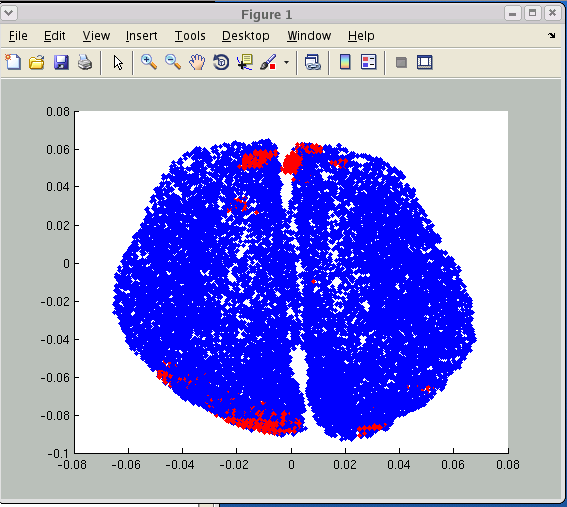
- If you use the normalization file (_sn.mat) for another subject, these positions will not match. In addition, you need to use the same T1 image for SPM analysis and FreeSurfer cortical surface extraction. Check that your _sn.mat file are created from the MR image of the subject you deal with.
- Otherwise, the problem may stem from the origin of the T1 image on which EPI images are registered. Load the T1 image on SPM.

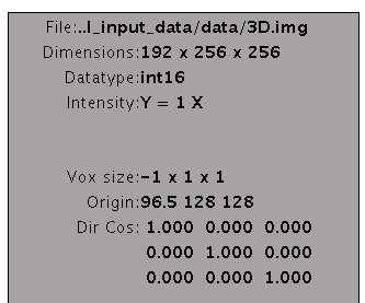
- Check the origin of the T1 image. If the origin does not the
center of the image, the voxel positions in the .spm.mat file can be
shifted, leading to a misalignment of the cortical surface model and
voxel positions on VBMEG. The following figure shows a valid T1 image.
The size of this image is 191x256x256.
- If the origin is not the center of the image, you may need to modify the header file. On SPM8 GUI, you can use "Reset" button.
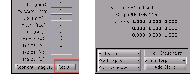
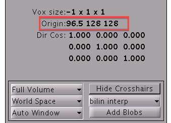
- Select the T1 image file in the file dialog. Then the origin will be set to the center of the T1 image.
- After reset the origin, you need to perform SPM precessing and make .spm.mat file again.
- You can check this by using the following MATLAB commands:
MATLAB Scripts
Add new area information into cortical area file (.area.mat)
Extract area on which some activity (e.g., t-value) is larger than a threshold
% files and ids
area_file = 'sbj.area.mat';
act_file = 'sbj.act.mat';

% thresholding
act = vb_get_act(act_file,'t_value'); % get activity map 't_value' stored in act_file
ix = find(a.xxP>=threshold);

% make and add new area
area_new.Iextract = ix; % thresholded area
area_new.key = 'area_new_id';  % any identifier
vb_add_area(area_file,area_new); % area_new is added to area_file
Concatenate two areas (union)
% files
area_file = 'sbj.area.mat';

% get areas
area1 = vb_get_area(area_file,'area1');
area2 = vb_get_area(area_file,'area2');

% concatenation
ix = union(area1.Iextract,area2.Iextract);

% make and add new area
area_new.Iextract = ix;
area_new.key = 'area_new_id';  % any identifier
vb_add_area(area_file,area_new); % area_new is added to area_file
Plot cortical surface model
Plot vertices of cortical surface model superimposed on the inflated model
% files
brain_file = 'sbj.brain.mat';

% plot cortical surface model
[V,F,tmp,inf_C] = vb_load_cortex(brain_file,'Inflate');
plot_parm        = vb_set_plot_parm;
vb_plot_cortex(plot_parm,V,F,inf_C,J);
hold on;

% vertex indices
ix = [1; 10; 100; 1000];

% plot vertices
plot3(V(ix,1),V(ix,2),V(ix,3),'r.');
Plot vertices of cortical surface model superimposed on the inflated model (left hemisphere only)
% files
brain_file = 'sbj.brain.mat';

% plot cortical surface model (left hemisphere only)
[V,F,tmp,inf_C] = vb_load_cortex(brain_file,'Inflate');
plot_parm = vb_set_plot_parm;
plot_parm.LRflag = 'L'; % 'L' for LH, 'R' for RH, 'LR' for both hemispheres
vb_plot_cortex(plot_parm,V,F,inf_C,J);
hold on;

% vertex indices
ix = [1; 10; 100; 1000];

% choose vertices of LH
ix_lh = F.F3L(:); % F.F3L(:) including vertex indices of LH
ix = intersect(ix,ix_lh);

% plot vertices
plot3(V(ix,1),V(ix,2),V(ix,3),'r.');
References
- Toda A, Imamizu H, Kawato M, Sato MA.(2011). Reconstruction of two-dimensional movement trajectories from selected magnetoencephalography cortical currents by combined sparse Bayesian methods. NeuroImage. 54(2), 892-905.
- 森重健一, 川脇大, 吉岡琢, 佐藤雅昭, 川人光男 (2010). 脳磁図逆問題における複数のアーチファクト源と脳内電流分布の同時推定法 電子情報通信学会論文誌, J93-D, 2, 127-138.
- Callan, D. E., Callan, A. M., Gamez, M., Sato, M., Kawato, M. (2010). Premotor cortex mediates perceptual performance. NeuroImage, 51, 2, 844-858.
- Morishige, K., Kawawaki, D., Yoshioka, T., Sato, M.A., Kawato, M. (2009). Artifact Removal Using Simultaneous Current Estimation of Noise and Cortical Sources. Lecture Notes in Computer Science: ICONIP 2008. Springer-Verlag, Berlin, pp. 335–342.
- Fujiwara, Y., Yamashita, O., Kawawaki, D., Doya, K., Kawato, M., Toyama, K., Sato, M. (2009). A hierarchical Bayesian method to resolve an inverse problem of MEG contaminated with eye movement artifacts. NeuroImage, 45, 2, 393-409.
- Yoshioka, T., Sato, M., Toyama, K., Yamashita, O., Nishina, S., Yamagishi, N., Kawato, M. (2008). Evaluation of hierarchical Bayesian method through retinotopic brain activities reconstruction from fMRI and MEG signals. NeuroImage, 42, Issue 4, 1397-1413.
- Shibata, K., Yamagishi, N., Goda, N., Yoshioka, T., Yamashita, O., Sato, M., Kawato, M. (2008). The Effects of feature attention on prestimulus cortical activity in the human visual system. Cerebral Cortex , Vol.18, 10, 1664-1675.
- Sato, M., Yoshioka, T., Kajiwara, S., Toyama, K., Goda, N., Doya, K., & Kawato, M. (2004). Hierarchical Bayesian estimation for MEG inverse problem. NeuroImage, 23, 806–826.
- Kajihara S, Ohtani Y, Goda N, Tanigawa M, Ejima Y, Toyama K. (2004). Wiener filter-magnetoencephalography of visual cortical activity. Brain Topogr. 2004 Fall;17(1):13-25.
Last update: 23 Aug 2012, taku-y