Connectome dynamics estimation tutorial
Contents
- Contents
- 0. Download
- 1. Introduction
- 2. Starting tutorial
- 3. Modeling brain to define current sources
- 4. Importing fMRI information
- 5. Source imaging from EEG data
- 6. Source imaging from MEG data
- 7. Source imaging from EEG-MEG data
- 8. Modeling connectome dynamics
0. Download
Tutorial data and programs (tutorial.zip)
1. Introduction
1.1. Scenario
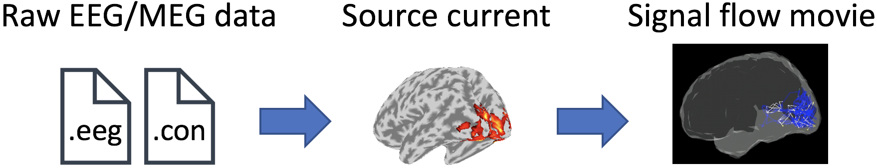
VBMEG allows us to reveal signal flows between brain regions that dynamically change in the order of milliseconds. Using the real experimental data, this tutorial guides through the procedures from importing the raw EEG/MEG data to creating movies displaying the signal flows. All the procedures will be conducted with scripts.
1.2. Experimental procedure
In the experiment, subjects performed three tasks:
- Auditory task,
- Somatosensory task,
- Visual task.
In the auditory task, the subjects were instructed to close their eyes and listen to a pure tone. The tone was presented to both of the ears. In the somatosensory task, the subjects were instructed to close their eyes and an electrical stimulation was presented to the right median nerve. In the visual task, the subjects were instructed to open their eyes and observe the concentric rings that expanded or contracted at 7 deg/s.
During the tasks, MEG and EEG were simultaneously recorded with a whole-head 400-channel system (210-channel Axial and 190-channel Planar Gradiometers; PQ1400RM; Yokogawa Electric Co., Japan) and a whole-head 63-channel system (BrainAmp; Brain Products GmbH, Germany), respectively. The sampling frequency was 1 kHz. Electrooculogram (EOG) signals were also simultaneously recorded and included in the EEG file.
Using three Tesla MR scanner (MAGNETOM Trio 3T; Siemens, Germany), we also conducted MRI experiment to obtain structural (T1), diffusion, and functional MRIs. The fMRI was recorded only during the visual task from a subject.
2. Starting tutorial
2.1. Setting environment
This tutorial was developed under MATLAB 2013b on Linux.
(1) Download and unzip tutorial.zip
(2) Copy and paste all the files to $your_dir
(3) Start MATLAB and change current directory to $your_dir/program
(4) Open tutorial.m by typing
>> open tutorial
2.2. Adding path
Thereafter, we will sequentially execute the commands in tutorial.m from the top.
We add paths to necessary toolboxes: VBMEG and SPM 8.
>> addpath(path_of_VBMEG);
>> vbmeg
>> addpath(path_of_SPM8);
You need to modify path_of_VBMEG and path_of_SPM8 for your environment.
2.3. Creating project
We set the parameters for analyzing the EEG and MEG data, and set the file and directory names.
>> sub = 's006';
>> p = create_project(sub);
You can also set sub = 's043'.
By default, analyzed data and figures will be respectively saved in
- $your_dir/analyzed_data/s006,
- $your_dir/figure.
3. Modeling brain to define current sources
First of all, we construct a cortical surface model from the T1 image and define current sources on it.
3.1. Importing T1 image
We convert T1 DICOM files to a NIfTI (.nii) file (User manual).
>> import_T1(p);
The following file will be saved.
- $your_dir/analyzed_data/s006/struct/Subject.nii
3.2. Correcting bias in T1 image
Using SPM, we correct bias in the T1 image (User manual).
>> correct_bias_in_T1(p);
The following file will be saved.
- $your_dir/analyzed_data/s006/struct/mSubject.nii
3.3. Segmenting T1 image
Using SPM, we extract a gray matter image from the T1 image.
>> segment_T1(p);
The following files will be saved.
- $your_dir/analyzed_data/s006/struct/c1mSubject.nii (Gray matter)
- $your_dir/analyzed_data/s006/struct/mSubject_seg_sn.mat (Normalization)
The gray matter image will be used in Preparing leadfield, and the normalization file will be used in 4. Importing fMRI information.
3.4. Constructing cortical surface models from T1 images
Using FreeSurfer, we construct a polygon model of a cortical surface from the T1 image (User manual).
>> construct_cortical_surface_model(p);
The generated files will be saved in
- $your_dir/analyzed_data/s006/freesurfer.
3.5. Constructing brain models from cortical surface models
From the cortical surface model, we construct a brain model, in which the positions of current sources are defined (vb_job_brain.m).
>> construct_brain_model(p);
The following files will be saved.
- $your_dir/analyzed_data/s006/brain/Subject.brain.mat (Brain model)
- $your_dir/analyzed_data/s006/brain/Subject.act.mat
In Subject.act.mat, the fMRI information will be stored (Importing fMRI information).
4. Importing fMRI information
4.1. Importing fMRI information
VBMEG estimates source currents from EEG/MEG data using an fMRI result as a prior on the source current variances. The fMRI result is assumed to be obtained using SPM 8. We import the fMRI result of the visual task (User manual, vb_job_fmri.m).
>> import_fmri(p);
T-values and percent signal changes will be stored in
- $your_dir/analyzed_data/s006/brain/Subject.act.mat.
4.2. Checking imported fMRI result
We check the imported fMRI result (vb_plot_cortex.m).
>> check_imported_fmri(p);
Figures will be saved in
- $your_dir/figure/check_imported_fmri.
5. Source imaging from EEG data
In this section, we introduce the procedures from importing the raw EEG data to the source current estimation.
5.1. Preprocessing
Importing EEG data
We convert BrainAmp files to MAT files (User manual, vb_job_meg.m).
>> import_eeg(p);
The following files will be saved.
- $your_dir/analyzed_data/s006/eeg/loaded/a1.eeg.mat (Auditory task, run 1)
- $your_dir/analyzed_data/s006/eeg/loaded/s1.eeg.mat (Somatosensory task, run 1)
- $your_dir/analyzed_data/s006/eeg/loaded/v1.eeg.mat (Visual task, run 1)
- $your_dir/analyzed_data/s006/eeg/loaded/v2.eeg.mat (Visual task, run 2)
Filtering EEG data
The recorded EEG data include drift and line noise (60 Hz at Kansai in Japan). To remove these noises, we apply a low-pass filter, down-sampling, and a high-pass filter.
>> filter_eeg(p);
The following files will be saved.
- $your_dir/analyzed_data/s006/eeg/filtered/a1.eeg.mat (Auditory task, run 1)
- $your_dir/analyzed_data/s006/eeg/filtered/s1.eeg.mat (Somatosensory task, run 1)
- $your_dir/analyzed_data/s006/eeg/filtered/v1.eeg.mat (Visual task, run 1)
- $your_dir/analyzed_data/s006/eeg/filtered/v2.eeg.mat (Visual task, run 2)
Making trial data
We segment the continuous EEG data into trials. First, we detect stimulus onsets from the trigger signals included in the EEG data. Then, we segment the EEG data into trials by the detected stimulus onsets.
>> make_trial_eeg(p);
The following files will be saved.
- $your_dir/analyzed_data/s006/eeg/trial/a1.eeg.mat (Auditory task, run 1)
- $your_dir/analyzed_data/s006/eeg/trial/s1.eeg.mat (Somatosensory task, run 1)
- $your_dir/analyzed_data/s006/eeg/trial/v1.eeg.mat (Visual task, run 1)
- $your_dir/analyzed_data/s006/eeg/trial/v2.eeg.mat (Visual task, run 2)
Detecting blinks from EOG data
We detect trials in which the subject blinked during the exposure to the visual stimulus based on the power of the EOG data. The detected trials will be rejected in Rejecting bad trials.
>> detect_blink_from_eog(p);
The blink information will be stored in EEGinfo in the above trial files.
Removing EOG components
We regress out EOG components from the EEG data. For each channel, we construct a linear model to predict the EEG data from the EOG data and remove the prediction from the EEG data.
>> regress_out_eog_from_eeg(p);
The following files will be saved.
- $your_dir/analyzed_data/s006/eeg/trial/r_a1.eeg.mat (Auditory task, run 1)
- $your_dir/analyzed_data/s006/eeg/trial/r_s1.eeg.mat (Somatosensory task, run 1)
- $your_dir/analyzed_data/s006/eeg/trial/r_v1.eeg.mat (Visual task, run 1)
- $your_dir/analyzed_data/s006/eeg/trial/r_v2.eeg.mat (Visual task, run 2)
Checking the result of removing EOG components
To check if the EOG components were correctly removed, we compare the spatial distributions of the powers between the original and the EOG-removed EEG data (vb_plot_sensor_2d.m).
>> check_removing_eog_from_eeg(p);
The following figure will be saved.
- $your_dir/figure/check_removing_eog_from_eeg/s006.png
Correcting baseline
For each channel and trial, we make the average of prestimulus EEG to 0.
>> correct_baseline_eeg(p);
The following files will be saved.
- $your_dir/analyzed_data/s006/eeg/trial/br_a1.eeg.mat (Auditory task, run 1)
- $your_dir/analyzed_data/s006/eeg/trial/br_s1.eeg.mat (Somatosensory task, run 1)
- $your_dir/analyzed_data/s006/eeg/trial/br_v1.eeg.mat (Visual task, run 1)
- $your_dir/analyzed_data/s006/eeg/trial/br_v2.eeg.mat (Visual task, run 2)
Combining trials across runs
To handle all the trials collectively, we combine the information of all the trials.
>> combine_trial_eeg(p);
The following file will be saved.
- $your_dir/analyzed_data/s006/eeg/trial/all.info.mat
This file contains the information (e.g. file paths) to serve as the shortcut to these files.
- br_a1.eeg.mat
- br_s1.eeg.mat
- br_v1.eeg.mat
- br_v2.eeg.mat
Applying independent component analysis (ICA)
Using EEGLAB, we apply ICA to the EEG data.
>> apply_ica_eeg(p);
The following file will be saved.
- $your_dir/analyzed_data/s006/eeg/ica/apply_ica_eeg.mat
Automatically classifying ICs
We automatically classify ICs into brain activities and noise based on kurtosis and entropy (Barbati et al., 2004).
>> classify_ic_eeg(p);
The following file will be saved.
- $your_dir/analyzed_data/s006/eeg/ica/classify_ic_eeg.mat
Manually correcting classification results
We manually correct the classification results based on the below conditions:
- the spatial patterns of the mixing matrices,
- the stimulus-triggered averages of the ICs,
- the power spectra of the ICs.
Therefore, this step requires your input.
>> correct_classify_ic_eeg(p);
The figure displaying the three conditions will appear. In this figure, brain and noise ICs are respectively represented by blue and red lines. You need to input IC number in the command window to correct or just push enter to go ahead. If you want to exit the correction, please input 0. For s006, you do not need to correct any ICs.
The following file will be saved.
- $your_dir/analyzed_data/s006/eeg/ica/correct_classify_ic_eeg.mat
Removing noise ICs
We remove the ICs classified as noise from the EEG data (Jung et al., 2001).
>> remove_noise_ic_eeg(p);
The following files will be saved.
- $your_dir/analyzed_data/s006/eeg/trial/i_all.info.mat (Shortcut to the following files)
- $your_dir/analyzed_data/s006/eeg/trial/ibr_a1.eeg.mat (Auditory task, run 1)
- $your_dir/analyzed_data/s006/eeg/trial/ibr_s1.eeg.mat (Somatosensory task, run 1)
- $your_dir/analyzed_data/s006/eeg/trial/ibr_v1.eeg.mat (Visual task, run 1)
- $your_dir/analyzed_data/s006/eeg/trial/ibr_v2.eeg.mat (Visual task, run 2)
Rejecting bad channels
We detect noisy channels based on the amplitudes of the EEG data and reject them. The rejected channels will not be used in the following analyses.
>> reject_channel_eeg(p);
The following file will be saved.
- $your_dir/analyzed_data/s006/eeg/trial/ri_all.info.mat
Rejecting bad trials
We reject the trials in which the subject blinked during the exposure to the visual stimulus. The rejected trials will not be used in the following analyses.
>> reject_trial_eeg(p);
The following file will be saved.
- $your_dir/analyzed_data/s006/eeg/trial/rri_all.info.mat
Taking common average
We take common average; that is, we make the averages of EEG data across the channels to 0.
>> common_average_eeg(p);
The following files will be saved.
- $your_dir/analyzed_data/s006/eeg/trial/crri_all.info.mat (Shortcut to the following files)
- $your_dir/analyzed_data/s006/eeg/trial/cibr_a1.eeg.mat (Auditory task, run 1)
- $your_dir/analyzed_data/s006/eeg/trial/cibr_s1.eeg.mat (Somatosensory task, run 1)
- $your_dir/analyzed_data/s006/eeg/trial/cibr_v1.eeg.mat (Visual task, run 1)
- $your_dir/analyzed_data/s006/eeg/trial/cibr_v2.eeg.mat (Visual task, run 2)
Separating trials into tasks
We separate the combined trials into the three tasks: the auditory, somatosensory, and visual tasks.
>> separate_eeg(p);
The following files will be saved.
- $your_dir/analyzed_data/s006/eeg/trial/crri_a.eeg.mat (Auditory task)
- $your_dir/analyzed_data/s006/eeg/trial/crri_s.eeg.mat (Somatosensory task)
- $your_dir/analyzed_data/s006/eeg/trial/crri_v.eeg.mat (Visual task)
Showing preprocessed EEG data
For each task, we show the processed EEG data averaged across the trials (vb_plot_sensor_2d.m).
>> show_trial_average_eeg(p);
Figures will be saved in
- $your_dir/figure/show_trial_average_eeg/006.
5.2. Source imaging
Preparing leadfield
First, we construct a 3-shell (cerebrospinal fluid, skull, and scalp) surface model (User manual, vb_job_head_3shell.m). Then, we make the leadfield matrix based on the 3-shell model (User manual, vb_job_leadfield.m). Finally, we take the common average of the leadfield matrix.
>> prepare_leadfield_eeg(p);
The following files will be saved.
- $your_dir/analyzed_data/s006/eeg/leadfield/Subject.head.mat (3-shell model)
- $your_dir/analyzed_data/s006/eeg/leadfield/Subject.basis.mat (Leadfield)
Estimating source currents
First, we estimate the current variance by integrating the fMRI information and the EEG data (User manual, vb_job_vb.m). Then, we estimate source currents using the current variance as a constraint (User manual, vb_job_current.m).
>> estimate_source_current_eeg(p);
The following files will be saved.
- $your_dir/analyzed_data/s006/eeg/current/a.bayes.mat (Current variance)
- $your_dir/analyzed_data/s006/eeg/current/a.curr.mat (Source current)
- $your_dir/analyzed_data/s006/eeg/current/s.bayes.mat
- $your_dir/analyzed_data/s006/eeg/current/s.curr.mat
- $your_dir/analyzed_data/s006/eeg/current/v.bayes.mat
- $your_dir/analyzed_data/s006/eeg/current/v.curr.mat
Showing estimated source currents
For each task, we show the estimated source currents averaged across the trials (vb_plot_cortex.m).
>> show_source_current_eeg(p);
Figures will be saved in
- $your_dir/figure/show_source_current_eeg/006.
6. Source imaging from MEG data
In this section, we introduce the procedures from importing the raw MEG data to the source current estimation.
6.1. Preprocessing
Importing MEG data
We convert Yokogawa MEG files to MAT files (User manual, vb_job_meg.m).
>> import_meg(p);
The following files will be saved.
- $your_dir/analyzed_data/s006/meg/loaded/a1.meg.mat (Auditory task, run 1)
- $your_dir/analyzed_data/s006/meg/loaded/s1.meg.mat (Somatosensory task, run 1)
- $your_dir/analyzed_data/s006/meg/loaded/v1.meg.mat (Visual task, run 1)
- $your_dir/analyzed_data/s006/meg/loaded/v2.meg.mat (Visual task, run 2)
Removing environmental noise
The MEG data include large environmental noise from air‐conditioner and others. Using reference sensor data, we remove the environmental noise from the MEG data (de Cheveigne and Simon, 2008).
>> remove_env_noise_meg(p);
The following files will be saved.
- $your_dir/analyzed_data/s006/meg/denoised/a1.meg.mat (Auditory task, run 1)
- $your_dir/analyzed_data/s006/meg/denoised/s1.meg.mat (Somatosensory task, run 1)
- $your_dir/analyzed_data/s006/meg/denoised/v1.meg.mat (Visual task, run 1)
- $your_dir/analyzed_data/s006/meg/denoised/v2.meg.mat (Visual task, run 2)
Checking the result of removing environmental noise
To check if the environmental noise is correctly removed, we compare the power spectra between the original and the noise-removed MEG data.
>> check_denoised_meg(p);
The following figure will be saved.
- $your_dir/figure/check_denoised_meg/006.png
Filtering MEG data
The recorded MEG data include drift and line noises (60 Hz at Kansai in Japan). To remove these noises, we apply a low-pass filter, down-sampling, and a high-pass filter.
>> filter_meg(p);
The following files will be saved.
- $your_dir/analyzed_data/s006/meg/filtered/a1.meg.mat (Auditory task, run 1)
- $your_dir/analyzed_data/s006/meg/filtered/s1.meg.mat (Somatosensory task, run 1)
- $your_dir/analyzed_data/s006/meg/filtered/v1.meg.mat (Visual task, run 1)
- $your_dir/analyzed_data/s006/meg/filtered/v2.meg.mat (Visual task, run 2)
Making trial data
We segment the continuous MEG data into trials. First, we detect stimulus onsets from the trigger signals included in the MEG data. Then, we segment the MEG data into trials by the detected stimulus onsets.
>> make_trial_meg(p);
The following files will be saved.
- $your_dir/analyzed_data/s006/meg/trial/a1.meg.mat (Auditory task, run 1)
- $your_dir/analyzed_data/s006/meg/trial/s1.meg.mat (Somatosensory task, run 1)
- $your_dir/analyzed_data/s006/meg/trial/v1.meg.mat (Visual task, run 1)
- $your_dir/analyzed_data/s006/meg/trial/v2.meg.mat (Visual task, run 2)
Importing blink information from EEG data
In the EEG analyses, we detected the trials in which the subject blinked during the exposure to the visual stimulus (Detecting blinks from EOG data). We import this blink information to the MEG data to reject the blink trials in Rejecting bad trials.
>> import_blink_from_eeg(p);
The blink information will be stored in MEGinfo in the above trial data.
Removing EOG components
We regress out EOG components from the MEG data. For each channel, we construct a linear model to predict the MEG data from the EOG data and remove the prediction from the MEG data.
>> regress_out_eog_from_meg(p);
The following files will be saved.
- $your_dir/analyzed_data/s006/meg/trial/r_a1.meg.mat (Auditory task, run 1)
- $your_dir/analyzed_data/s006/meg/trial/r_s1.meg.mat (Somatosensory task, run 1)
- $your_dir/analyzed_data/s006/meg/trial/r_v1.meg.mat (Visual task, run 1)
- $your_dir/analyzed_data/s006/meg/trial/r_v2.meg.mat (Visual task, run 2)
Checking the result of removing EOG components
To check if the EOG components were correctly removed, we compare the spatial distributions of the powers between the original and the EOG-removed MEG data (vb_plot_sensor_2d.m).
>> check_removing_eog_from_meg(p);
The following figure will be saved.
- $your_dir/figure/check_removing_eog_from_meg/s006.png
Correcting baseline
For each channel and trial, we make the average of prestimulus MEG to 0.
>> correct_baseline_meg(p);
The following files will be saved.
- $your_dir/analyzed_data/s006/meg/trial/br_a1.meg.mat (Auditory task, run 1)
- $your_dir/analyzed_data/s006/meg/trial/br_s1.meg.mat (Somatosensory task, run 1)
- $your_dir/analyzed_data/s006/meg/trial/br_v1.meg.mat (Visual task, run 1)
- $your_dir/analyzed_data/s006/meg/trial/br_v2.meg.mat (Visual task, run 2)
Combining trials across runs
To handle all the trials collectively, we combine the information of all the trials.
>> combine_trial_meg(p);
The following file will be saved.
- $your_dir/analyzed_data/s006/meg/trial/all.info.mat
This file contains the information (e.g. file paths) to serve as the shortcut to these files.
- br_a1.meg.mat
- br_s1.meg.mat
- br_v1.meg.mat
- br_v2.meg.mat
Applying ICA
Using EEGLAB, we apply ICA to the MEG data.
>> apply_ica_meg(p);
The following file will be saved.
- $your_dir/analyzed_data/s006/meg/ica/apply_ica_meg.mat
Automatically classifying ICs
We automatically classify ICs into brain activities and noise based on kurtosis and entropy (Barbati et al., 2004).
>> classify_ic_meg(p);
The following file will be saved.
- $your_dir/analyzed_data/s006/meg/ica/classify_ic_meg.mat
Manually correcting classification results
We manually correct the classification results based on the below conditions:
- the spatial patterns of the mixing matrices,
- the stimulus-triggered averages of the ICs,
- the power spectra of the ICs.
Therefore, this step requires your input.
>> correct_classify_ic_meg(p);
The figure displaying the three conditions will appear. In this figure, brain and noise ICs are respectively represented by blue and red lines. You need to input IC number in the command window to correct or just push enter to go ahead. If you want to exit the correction, please input 0. For s006, you need to correct an IC (maybe IC 5) to the brain activity because it exhibits a clear stimulus-evoked response.
The following file will be saved.
- $your_dir/analyzed_data/s006/meg/ica/correct_classify_ic_meg.mat
Removing noise ICs
We remove the ICs classified as noise from the MEG data (Jung et al., 2001).
>> remove_noise_ic_meg(p);
The following files will be saved.
- $your_dir/analyzed_data/s006/meg/trial/i_all.info.mat (Shortcut to the following files)
- $your_dir/analyzed_data/s006/meg/trial/ibr_a1.meg.mat (Auditory task, run 1)
- $your_dir/analyzed_data/s006/meg/trial/ibr_s1.meg.mat (Somatosensory task, run 1)
- $your_dir/analyzed_data/s006/meg/trial/ibr_v1.meg.mat (Visual task, run 1)
- $your_dir/analyzed_data/s006/meg/trial/ibr_v2.meg.mat (Visual task, run 2)
Rejecting bad channels
We detect noisy channels based on the amplitudes of the MEG data and reject them. The rejected channels will not be used in the following analyses.
>> reject_channel_meg(p);
The following file will be saved.
- $your_dir/analyzed_data/s006/meg/trial/ri_all.info.mat
Rejecting bad trials
We reject the trials in which the subject blinked during the exposure to the visual stimulus. The rejected trials will not be used in the following analyses.
>> reject_trial_meg(p);
The following file will be saved.
- $your_dir/analyzed_data/s006/meg/trial/rri_all.info.mat
Separating trials into tasks
We separate the combined trials into the three tasks: the auditory, somatosensory, and visual tasks.
>> separate_meg(p);
The following files will be saved.
- $your_dir/analyzed_data/s006/meg/trial/rri_a.meg.mat (Auditory task)
- $your_dir/analyzed_data/s006/meg/trial/rri_s.meg.mat (Somatosensory task)
- $your_dir/analyzed_data/s006/meg/trial/rri_v.meg.mat (Visual task)
Showing preprocessed MEG data
For each task, we show the processed MEG data averaged across the trials (vb_plot_sensor_2d.m).
>> show_trial_average_meg(p);
Figures will be saved in
- $your_dir/figure/show_source_current_meg/s006.
6.2. Source imaging
Preparing leadfield
First, we construct a 1-shell (cerebrospinal fluid) surface model (User manual, vb_job_head_3shell.m). Then, we make the leadfield matrix based on the 1-shell model (User manual, vb_job_leadfield.m).
>> prepare_leadfield_meg(p);
The following files will be saved.
- $your_dir/analyzed_data/s006/meg/leadfield/Subject.head.mat (1-shell model)
- $your_dir/analyzed_data/s006/meg/leadfield/Subject.basis.mat (Leadfield)
Estimating source currents
First, we estimate the current variance by integrating the fMRI information and the MEG data (User manual, vb_job_vb.m). Then, we estimate source currents using the current variance as a constraint (User manual, vb_job_current.m).
>> estimate_source_current_meg(p);
The following files will be saved.
- $your_dir/analyzed_data/s006/meg/current/a.bayes.mat (Current variance)
- $your_dir/analyzed_data/s006/meg/current/a.curr.mat (Source current)
- $your_dir/analyzed_data/s006/meg/current/s.bayes.mat
- $your_dir/analyzed_data/s006/meg/current/s.curr.mat
- $your_dir/analyzed_data/s006/meg/current/v.bayes.mat
- $your_dir/analyzed_data/s006/meg/current/v.curr.mat
Showing estimated source currents
For each task, we show the estimated source currents averaged across the trials (vb_plot_cortex.m).
>> show_source_current_meg(p);
Figures will be saved in.
- $your_dir/figure/show_source_current_meg/006.
7. Source imaging from EEG-MEG data
Using VBMEG, we can estimate source currents from both of EEG and MEG data.
7.1. Estimating source currents
From the preprocessed EEG and MEG data and their leadfield matrices, we estimate the current variance. Then, we estimate source current using the current variance as a constraint.
>> estimate_source_current_meeg(p);
The following files will be saved.
- $your_dir/analyzed_data/s006/meeg/current/a.bayes.mat (Current variance)
- $your_dir/analyzed_data/s006/meeg/current/a.curr.mat (Source current)
- $your_dir/analyzed_data/s006/meeg/current/s.bayes.mat
- $your_dir/analyzed_data/s006/meeg/current/s.curr.mat
- $your_dir/analyzed_data/s006/meeg/current/v.bayes.mat
- $your_dir/analyzed_data/s006/meeg/current/v.curr.mat
7.2. Showing estimated source currents
For each task, we show the estimated source currents averaged across the trials (vb_plot_cortex.m).
>> show_source_current_meeg(p);
Figures will be saved in.
- $your_dir/figure/show_source_current_meeg/006.
8. Modeling connectome dynamics
In this section, we introduce procedures to model connectome dynamics from the source currents estimated from the MEG data (User manual).
8.1. dMRI processing
To obtain an anatomical connectivity, which is used as a constraint for modeling connectome dynamics, we analyze the dMRI using FSL and MRtrix (User manual). The required environment for this dMRI processing is described in this document. You need to modify p.process_host, which specifies the list of host names, for your environment.
Extracting brain from T1 image
We extract the brain (delete non-brain tissues) from the T1 image.
>> extract_brain_from_T1(p);
The following files will be saved.
- $your_dir/analyzed_data/s006/dmri/struct/Subject.nii.gz
- $your_dir/analyzed_data/s006/dmri/struct/Subject_brain.nii.gz
- $your_dir/analyzed_data/s006/dmri/struct/Subject_brain_mask.nii.gz
Importing dMRI
We convert dMRI DICOM files to a NIfTI (.nii.gz) file.
>> import_dmri(p);
The following files will be saved.
- $your_dir/analyzed_data/s006/dmri/dmri/data_dmri.nii.gz
- $your_dir/analyzed_data/s006/dmri/dmri/data_dmri.bval
- $your_dir/analyzed_data/s006/dmri/dmri/data_dmri.bvec
Correcting motion in dMRI
We correct motion in the dMRI.
>> correct_motion_in_dmri(p);
The following files will be saved.
- $your_dir/analyzed_data/s006/dmri/dmri/data_dmri_m.nii.gz
- $your_dir/analyzed_data/s006/dmri/dmri/data_dmri_m.bval
- $your_dir/analyzed_data/s006/dmri/dmri/data_dmri_m.bvec
Extracting brains from dMRI
We extract the brain (delete non-brain tissues) from the dMRI.
>> extract_brain_from_dmri(p);
The following file will be saved.
- $your_dir/analyzed_data/s006/dmri/dmri/data_dmri_m_brain_mask.nii.gz
Creating Fractional Anisotropy (FA) images from dMRI
We create an FA image from the dMRI.
>> create_fa_from_dmri(p);
The following file will be saved.
- $your_dir/analyzed_data/s006/dmri/dmri/data_FA_coreg.nii.gz
Coregistering T1 and cortical surface models to FA images
We coregister the T1 image and the cortical surface model to the FA images.
>> coregister_images(p);
The generated files will be saved in
- $your_dir/analyzed_data/s006/dmri/transwarp_info.
Removing noise in FA image
We remove the ambient noise in the FA image using the brain mask extracted from the T1 image.
>> remove_noise_in_fa(p);
The following file will be saved.
- $your_dir/analyzed_data/s006/dmri/dmri/data_FA.nii.gz
Parceling cortical surfaces
To define the seed and target region of interests (ROIs) used for fiber tracking, we parcel the cortical surface model.
>> parcel_cortical_surface(p);
The following file will be saved.
- $your_dir/analyzed_data/s006/dmri/parcels/parcels.mat
Parceling FA images based on parceled cortical surfaces
Based on the parceled cortical surface, we parcel the FA volume image.
>> parcel_fa_volume(p);
The generated files will be saved in
- $your_dir/analyzed_data/s006/dmri/parcels.
Creating masks for fiber tracking
We create a white matter volume file for fiber tracking.
>> create_mask_for_fiber_tracking(p);
Calculating fiber orientation density functions (FODF)
We calculate the FODF from the dMRI.
>> calculate_fodf(p);
The following files will be saved.
- $your_dir/analyzed_data/s006/dmri/fibertrack/wm.nii.gz (White matter)
- $your_dir/analyzed_data/s006/dmri/fibertrack/parcel_wm.nii.gz (Area mask)
Executing fiber tracking
Based on the FODF, we execute fiber tracking.
>> fiber_tracking(p);
The following file will be saved.
- $your_dir/analyzed_data/s006/dmri/fibertrack/anat_matrix.mat
Calculating connectivities
From the result of the fiber tracking, we calculate a binary connectivity matrix. Furthermore, we calculate the time lags between the ROIs based on the fiber lengths.
>> calculate_connectivity(p);
The following file will be saved.
- $your_dir/analyzed_data/s006/dmri/connectivity/connectivity.dmri.mat
- $your_dir/analyzed_data/s006/brain/Subject_dmri.area.mat
In Subject_dmri.area.mat, the ROI information, which vertex belongs to which ROI, is included.
Showing connectivity
We show the estimated connectivity.
>> show_connectivity(p);
The following figures will be saved.
- $your_dir/figure/show_connectivity/s006/brain.png (Connectivity on the brain)
- $your_dir/figure/show_connectivity/s006/matrix.png (Connectivity matrix)
8.2. Modeling connectome dynamics
From the source current estimated from the MEG data and the connectivity matrix, we estimate a linear dynamics model (Connectome dynamics estimation).
Calculating ROI-current
We estimate a linear dynamics model between the ROIs defined in the dMRI processing. Therefore, we calculate ROI-current by averaging the source currents within each ROI.
>> calculate_roi_current(p);
The following files will be saved.
- $your_dir/analyzed_data/s006/dynamics/roi_current/a.mat (Auditory task)
- $your_dir/analyzed_data/s006/dynamics/roi_current/s.mat (Somatosensory task)
- $your_dir/analyzed_data/s006/dynamics/roi_current/v.mat (Visual task)
Estimating dynamics model
From the ROI-current, we estimate a linear dynamics model using the L2-regularized least squares method, and in this model only the anatomically connected pairs of the ROIs have connectivity coefficients (Connectome dynamics estimation).
>> estimate_dynamics_model(p);
The following files will be saved.
- $your_dir/analyzed_data/s006/dynamics/model/a.lcd.mat (Auditory task)
- $your_dir/analyzed_data/s006/dynamics/model/s.lcd.mat (Somatosensory task)
- $your_dir/analyzed_data/s006/dynamics/model/v.lcd.mat (Visual task)
8.3. Creating movie
We create the movies displaying the signal flows between the ROIs (User manual).
Preparing input for creating movie
To create the movie, we need
- The ROI-current,
- The dynamics model,
- The place of the ROIs,
- Time information.
We gather these from separate files.
>> prepare_input_for_movie(p);
The following files will be saved.
- $your_dir/analyzed_data/dynamics/input_for_movie/a.mat (Auditory task)
- $your_dir/analyzed_data/dynamics/input_for_movie/s.mat (Somatosensory task)
- $your_dir/analyzed_data/dynamics/input_for_movie/v.mat (Visual task)
Executing fiber tracking
For the important pairs of the ROIs, we execute the fiber tracking again to obtain the shapes of the fibers.
>> fiber_tracking_for_movie(p);
The following files will be saved.
- $your_dir/analyzed_data/s006/dynamics/fibertrack/a/Vmni_connect.mat (Auditory task)
- $your_dir/analyzed_data/s006/dynamics/fibertrack/s/Vmni_connect.mat (Somatosensory task)
- $your_dir/analyzed_data/s006/dynamics/fibertrack/v/Vmni_connect.mat (Visual task)
Creating movie
We create the movies displaying the signal flows.
>> create_movie(p);
The following files will be saved.
- $your_dir/analyzed_data/s006/dynamics/movie/a/movie.avi (Auditory task)
- $your_dir/analyzed_data/s006/dynamics/movie/s/movie.avi (Somatosensory task)
- $your_dir/analyzed_data/s006/dynamics/movie/v/movie.avi (Visual task)
Congratulations! You have successfully achieved the goal of this tutorial.