VBMEG Tutorial(English)

• VBMEG Tutorial
  • Introduction
    • Files to be prepared
      • MEG Data file
      • Sensor alignment file
      • Details of MRI structure image file
      • Details of cortical model file
  • Directory
• Procedures
  • Setting a path
  • Creating project
  • Importing a cortical model
  • Importing MEG data
  • Calculating leadfield
  • Estimating current variance
  • Calculating current
  • Viewing estimated current

VBMEG Tutorial _

Introduction _

VBMEG is a Matlab toolbox used to estimate the cortical current from MEG and EEG data. This tutorial aims to understand how VBMEG processes data through the analysis of a sample data set.

Files to be prepared _

Tutorial data can be downloaded from http://vbmeg.atr.jp/?lang=en#DOWNLOAD

• MEG data file(A008a_BC_0.5HPF_100LPF_trig437_label4.ave)
• Sensor alignment file(marker1.pos.mat)
• Structural MRI image file(3D.hdr, 3D.img)
• Cortical model file(lh.(curv/inflated/smoothwm).asc, rh.(curv.inflated/smoothwm).asc)

MEG Data file _

• MEG data file(Yokogawa Electric Corporation format)
• Auditory stimuli task
• Averaged brain activity when a 3.2 kHz pure tone is presented to the left ear

Sensor alignment file _

• Information file to align MEG sensor coordinate system with subject’s structural MRI image coordinate system
• Created by the alignment program

Details of MRI structure image file _

• Analyze 7.5 format.The data sequence is left hand system (LAS).

  Refer to the following:
  http://www.wideman-one.com/gw/brain/orientation/orientterms.htm

Details of cortical model file _

• Individual cortical file created by FreeSurfer(http://surfer.nmr.mgh.harvard.edu/)
• Can be created from the structural MRI image file

Directory _

• Programs and input data are assumed to be stored as following:

D:\vbmeg(VBMEG program directory)
D:\data(input data directory)
│   3D.hdr
│   3D.img
│
├───FS
│       lh.curv.asc
│       lh.inflated.asc
│       lh.smoothwm.asc
│       rh.curv.asc
│       rh.inflated.asc
│       rh.smoothwm.asc
│
└───Yokogawa
        A008a_BC_0.5HPF_100LPF_trig437_label4.ave
        marker1.pos.mat

Procedures _

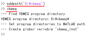
Setting a path _

• Start MATLAB and load VBMEG as follows:

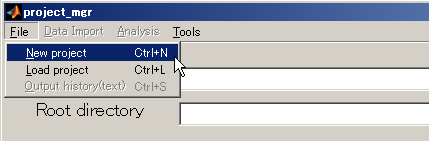
Creating project _

1. Start project_mgr from command line.

   >> project_mgr

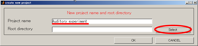
2. Select [File]->[New project].

   
   
   

3. Input project name and click the select button.

   
   
   

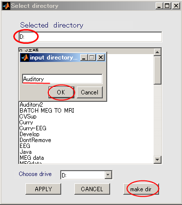
4. Change current directory to "D:". When you press the "make dir" button the dialog to input the name of the directory appears. Input "Auditory" and press the OK button.

   
   
   

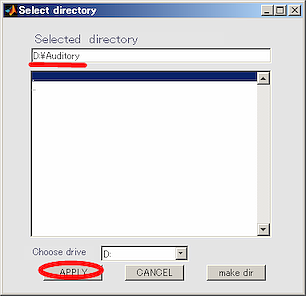
5. Select the working directory(D:\Auditory) in the dialog that appears, and click Apply button.

   
   
   

6. Press OK button and close the dialog.

   
   
   

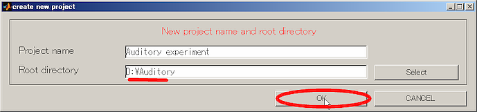
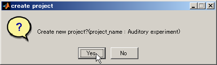
7. Select YES in the cofirmation dialog that appears.

   
   
   

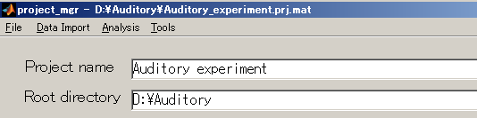
8. project_mgr is ready.

   
   
   

Importing a cortical model _

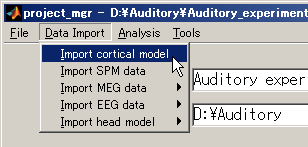
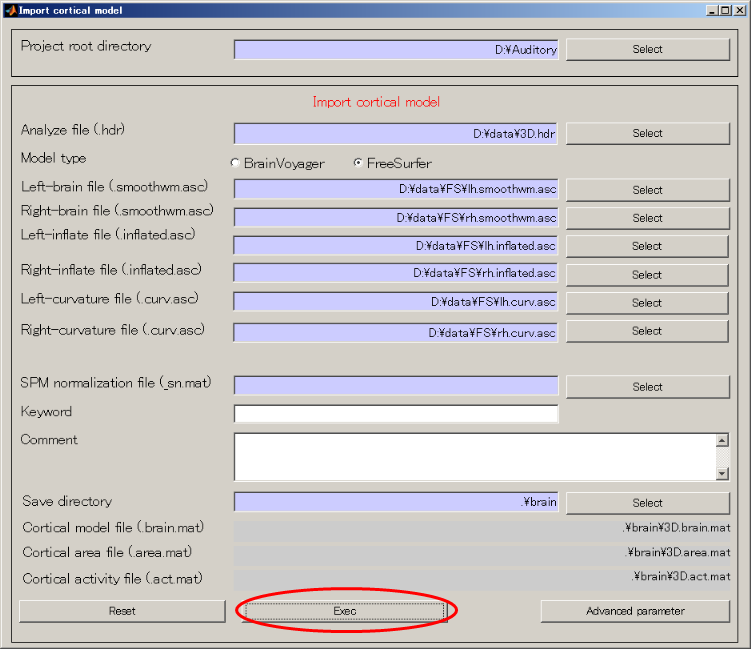
1. Select [Data Import]->[Import cortical model].

   
   
   

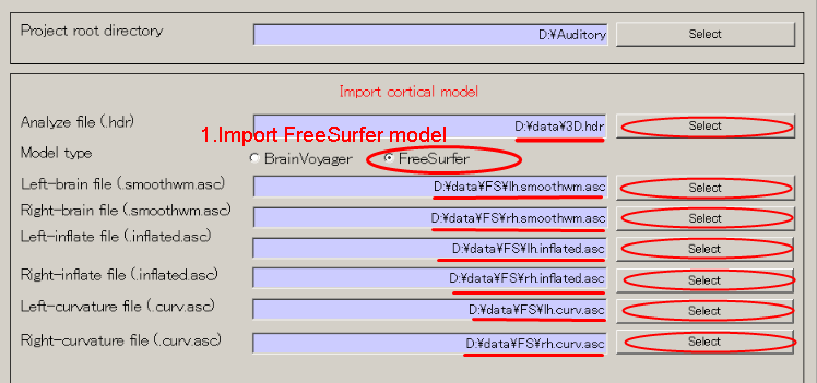
2. Set structural MRI image file and cortical model file(Press radio button: "FreeSurfer" first and then press the SELECT button to select the file for each subsequent field.)

   
   
   

3. Specifying output directory (D:\Auditory\brain)
   • Press Select button.

   
   
   

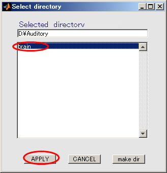
   • When you press the "make dir" button the dialog to input the name of the directory appears. Input "brain" and press the OK button.

   
   
   

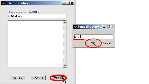
   • Click "brain" and press Apply.

   
   
   

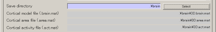
   • The output file name is updated.

   
   
   

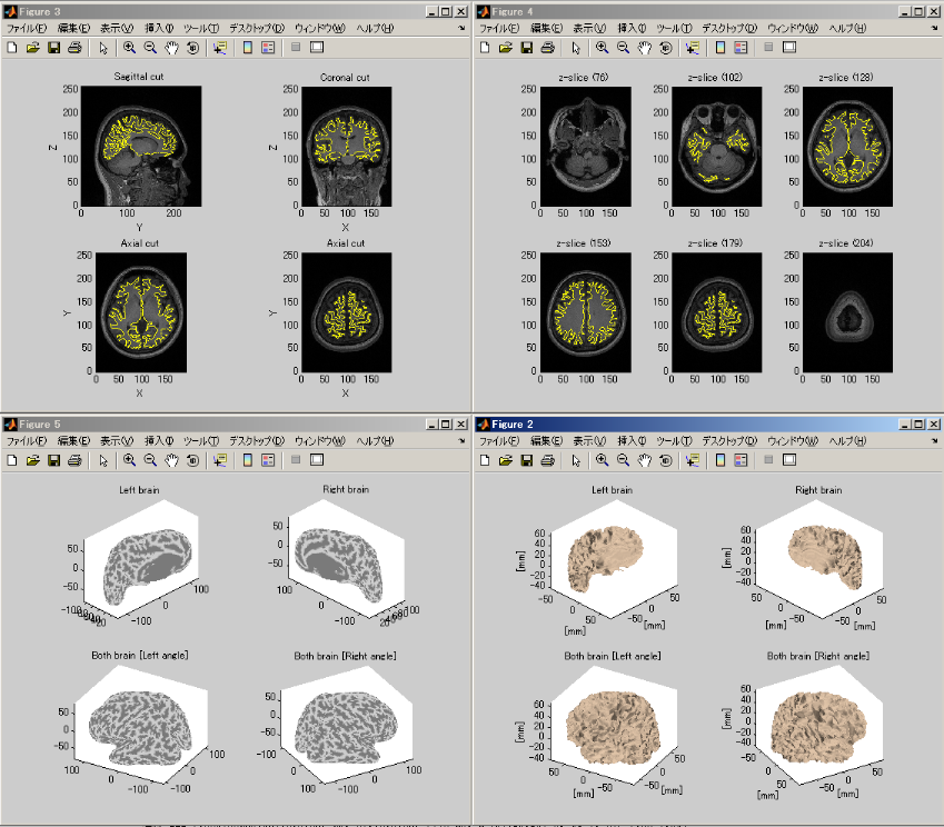
4. Press Exec button and wait for approximately 20 minutes. When the importation of cortical model is complete the results will be displayed.

   
   
   The following figure shows the displayed results.
   
   
   

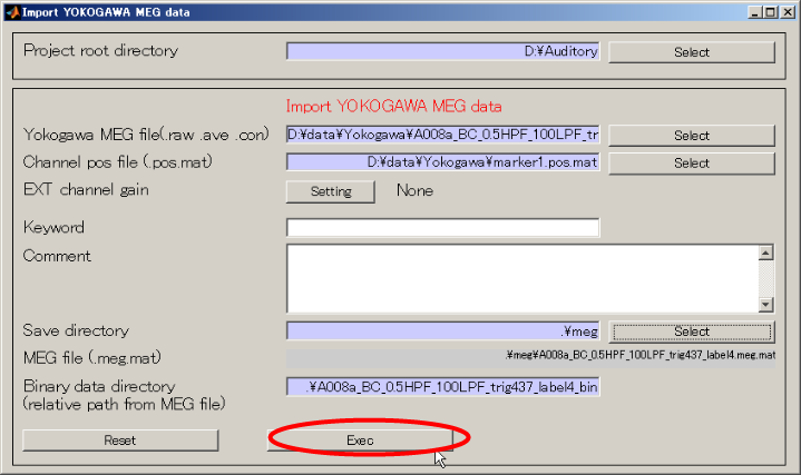
Importing MEG data _

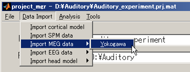
1. Select [Data Import]->[Import MEG data]->[Yokogawa].

   
   
   

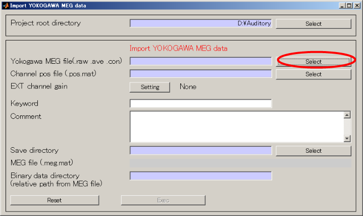
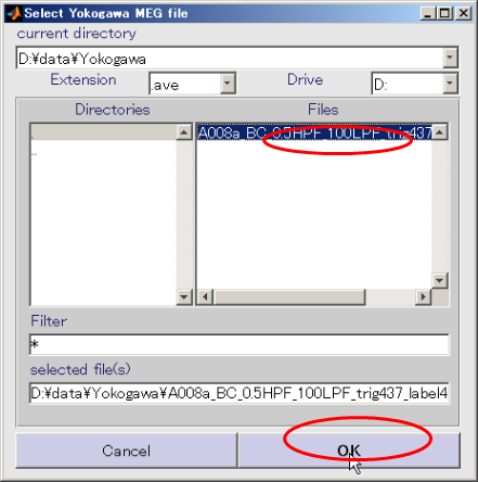
2. Specify Yokogawa MEG file.

   
   
   

3. Change the extension to .ave

   
   
   

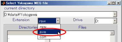
4. Select Yokogawa MEG file and press OK.(D:\data\Yokogawa\A008aBC0.5HPF100LPFtrig437_label4.ave)

   
   
   

5. Press select button and select sensor alignment file(D:\data\Yokogawa\marker1.pos.mat).

   
   
   

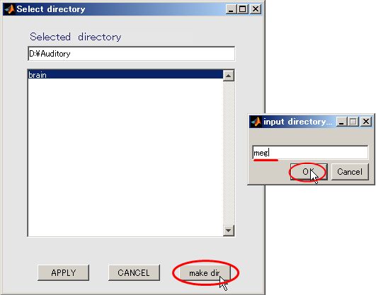
6. Create output destination(D:\Auditory\meg).
   • Press the Select button.

   
   
   

   • When you press the "make dir" button the dialog to input the name of the directory appears. Input "meg" and press the OK button.

   
   
   

   • Click "meg" and press APPLY.

   
   
   

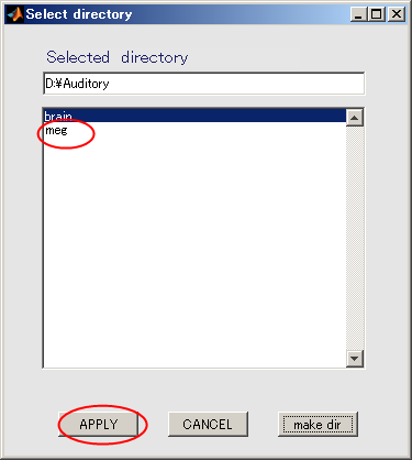
   • The output file name is updated.

   
   
   

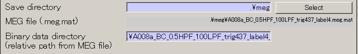
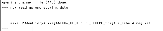
7. Press Exec button. The MEG data import will be completed in approximately 10 seconds.

   
   
   <<MATLAB Command window>>
   
   
   

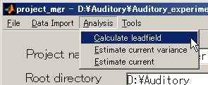
Calculating leadfield _

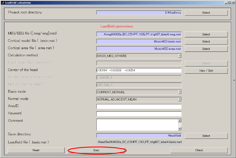
1. Select [Analysis]->[Calculate leadfield].

   
   
   

2. Specify MEG file(D:\Auditory\meg\A008a_BC_0.5HPF_100LPF_trig437_label4.meg.mat).

   
   
   

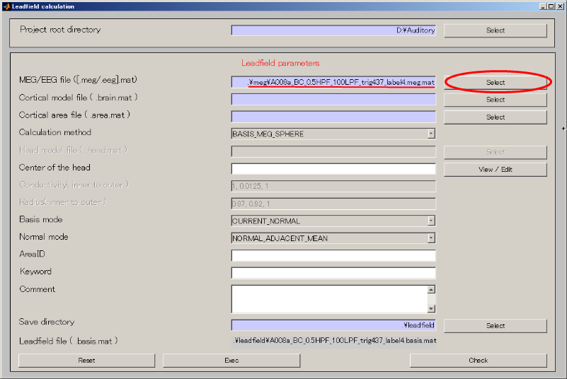
3. Specify Cortical model file(D:\Auditory\brain\3D.brain.mat).

   
   
   

4. Specify Cortical area file(D:\Auditory\brain\3D.area.mat).

   
   
   

5. Create output destination(D:\Auditory\leadfield).
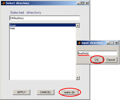
   • Push Select button.

   
   
   

   • When you press the "make dir" button the dialog to input the name of the directory appears. Input "leadfield" and press the OK button.

   
   
   

   • Click "leadfield" and press APPLY.

   
   
   

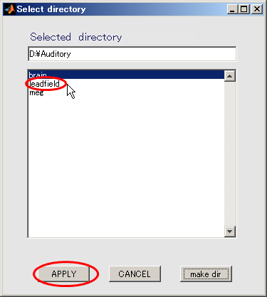
   • The output file name is updated.

   
   
   

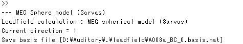
6. Press Exec button. The leadfield calculation will be completed in 20 to 30 seconds.

   
   
   <<MATLAB Command window>>
   
   
   

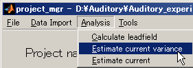
Estimating current variance _

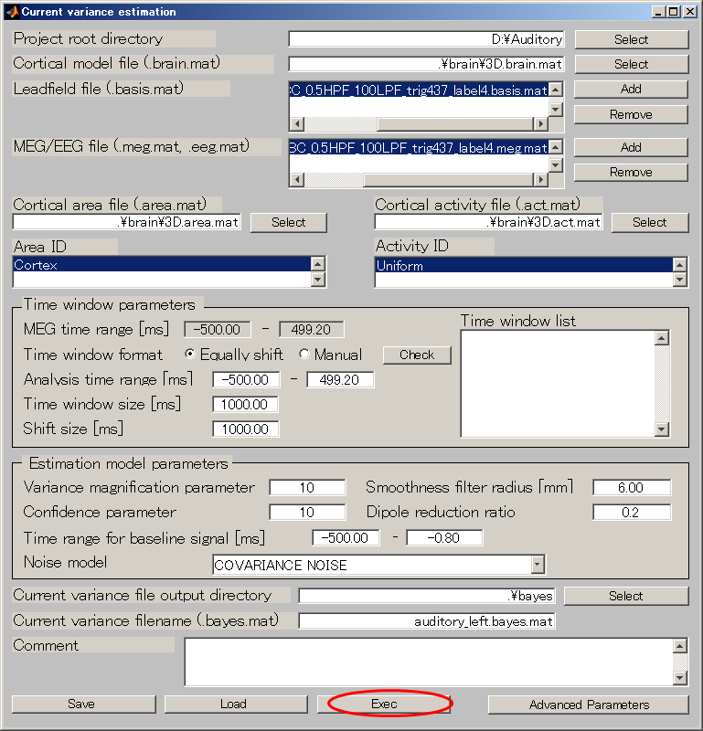
1. Select [Analysis]->[Estimate current variance].

   
   
   

2. Specify Cortical model file(D:\Auditory\brain\3D.brain.mat).

   
   
   

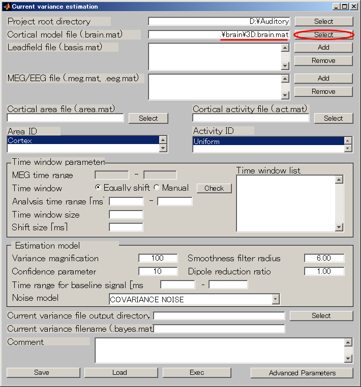
3. Specify Leadfield file(D:\Auditory\leadfield\A008a_BC_0.5HPF_100LPF_trig437_label4.basis.mat).

   
   
   

4. Specify MEG file(D:\Auditory\meg\A008a_BC_0.5HPF_100LPF_trig437_label4.meg.mat).

   
   
   

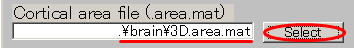
5. Specify Cortical area file(D:\Auditory\brain\3D.area.mat).

   
   
   

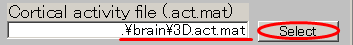
6. Specify Cortical activity file(D:\Auditory\brain\3D.act.mat).

   
   
   

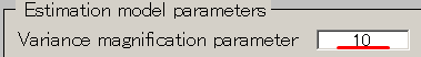
7. Set the Variance magnification parameter to 10.

   
   
   

8. Set the Dipole reduction ratio to 0.2.

   
   
   

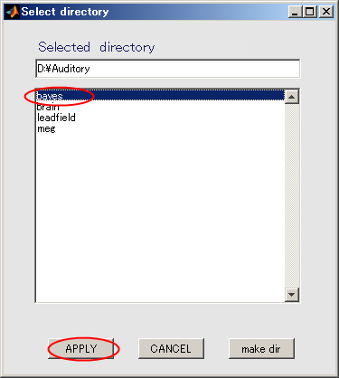
9. Create output destination(D:\Auditory\bayes).
   • Press Selectbutton.

   
   
   

   • When you press the "make dir" button the dialog to input the name of the directory appears. Input "bayes" and press the OK button.

   
   
   

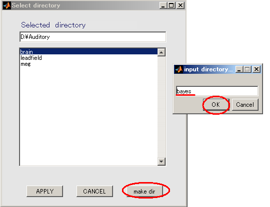
   • Click "bayes" and press APPLY.

   
   
   

10. Input the name of the output file.

    auditory_left[ENTER] will make it possible to add the extension:.bayes.mat automatically to the file name.
    
    
    

11. Press "Exec" button and the estimate will be complete in approximately 20 minutes.

    
    
    <<MATLAB Command Window>>
    

    Noise model: full covariance
    Load MEG data for noise estimate [D:\Auditory\.\meg\A008a_BC_0.5HPF_100LPF_trig437_label4.meg.mat]
    Session 1: -499.2 - 0.0[ms]
    Number of basis files (= Number of sessions): 1
    Area ID: Cortex
    Number of vertices: 20004
    --- Reduce cortex
    Number of reduced vertices: 4004
    --- Spatial smoothing filter calculation
    R = 6.00e-003, Rmax= 1.20e-002
    Number of vertices = 4004
    Number of vertices in expanded area = 20002
    Basis file for session 1: D:\Auditory\.\leadfield\A008a_BC_0.5HPF_100LPF_trig437_label4.basis.mat
    Number of basis files (= Number of sessions): 1
    Area ID: Cortex
    Number of vertices: 20004
    --- Reduce cortex
    Number of reduced vertices: 4004
    --- Spatial smoothing filter calculation
    R = 6.00e-003, Rmax= 1.20e-002
    Number of vertices = 4004
    Number of vertices in expanded area = 20002
    Basis file for session 1: D:\Auditory\.\leadfield\A008a_BC_0.5HPF_100LPF_trig437_label4.basis.mat
    Number of sessions: 1
    Time window: [1 1250]
    MEG data file for session 1: D:\Auditory\.\meg\A008a_BC_0.5HPF_100LPF_trig437_label4.meg.mat
    Number of sensors           : 400
    Number of trials            : 1
    --- Check variable consistency is OK
    Noise model: spherical
    Load MEG data for noise estimate [D:\Auditory\.\meg\A008a_BC_0.5HPF_100LPF_trig437_label4.meg.mat]
    Session 1: -499.2 - 0.0[ms]
    Number of sessions: 1
    Time window: [1 625]
    MEG data file for session 1: D:\Auditory\.\meg\A008a_BC_0.5HPF_100LPF_trig437_label4.meg.mat
    Number of sensors           : 400
    Number of trials            : 1
    --- Initial VB-update iteration = 100
    --- Total update iteration      = 100
    Sensor noise variance is estimated
    Background current variance is estimated
    Set prior fMRI activity pattern

    --- New VBMEG estimation program ---

    --- Initial VB-update iteration = 1000
    --- Total update iteration      = 1000
    Tn=  1, Iter=  50, FE=16183629.600099, Error=5.920164e-002
    Tn=  1, Iter= 100, FE=16184064.896437, Error=5.940531e-002
    Tn=  1, Iter= 150, FE=16184112.004743, Error=5.944172e-002
    Tn=  1, Iter= 200, FE=16184140.401725, Error=5.944495e-002
    Tn=  1, Iter= 250, FE=16184143.926441, Error=5.944783e-002
    Tn=  1, Iter= 300, FE=16184144.942685, Error=5.944801e-002
    Tn=  1, Iter= 350, FE=16184145.363067, Error=5.944747e-002
    Tn=  1, Iter= 400, FE=16184145.588821, Error=5.944667e-002
    Tn=  1, Iter= 450, FE=16184145.749733, Error=5.944572e-002
    Tn=  1, Iter= 500, FE=16184145.890986, Error=5.944465e-002
    Tn=  1, Iter= 550, FE=16184146.025482, Error=5.944347e-002
    Tn=  1, Iter= 600, FE=16184146.152109, Error=5.944222e-002
    Tn=  1, Iter= 650, FE=16184146.263429, Error=5.944096e-002
    Tn=  1, Iter= 700, FE=16184146.351531, Error=5.943978e-002
    Tn=  1, Iter= 750, FE=16184146.413128, Error=5.943876e-002
    Tn=  1, Iter= 800, FE=16184146.451154, Error=5.943794e-002
    Tn=  1, Iter= 850, FE=16184146.472196, Error=5.943733e-002
    Tn=  1, Iter= 900, FE=16184146.482881, Error=5.943690e-002
    Tn=  1, Iter= 950, FE=16184146.487982, Error=5.943661e-002
    Tn=  1, Iter=1000, FE=16184146.490319, Error=5.943642e-002
    Alpha is scaled back by bsnorm
    ----- Save estimation result in D:\Auditory\.\bayes\auditory_left.bayes.mat

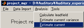
Calculating current _

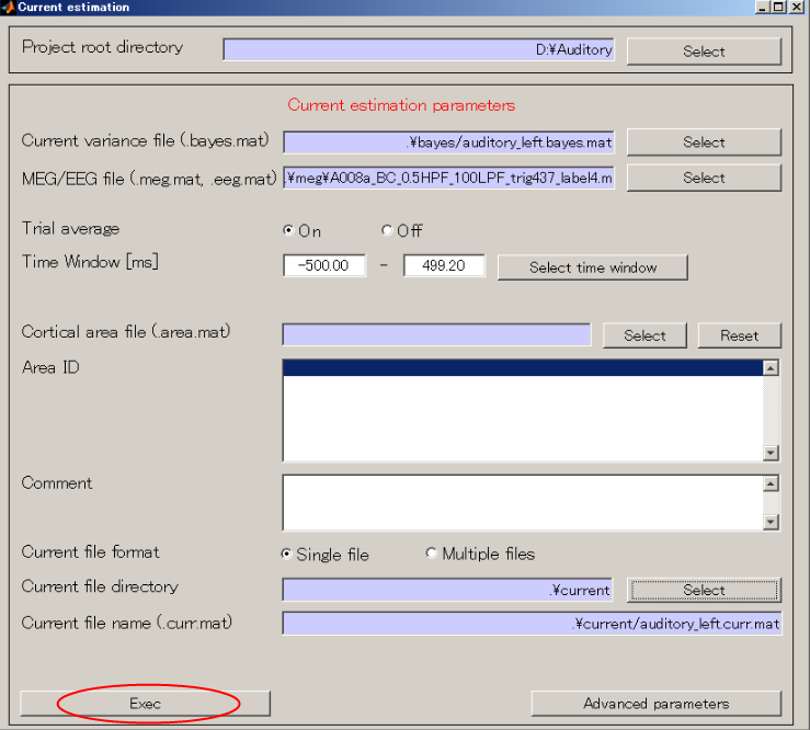
1. Select [Analysis]->[Estimate current].

   
   
   

2. Specify the current variance file(D:\Auditory\bayes\auditory_left.bayes.mat).

   The MEG file is set automatically.
   
   
   

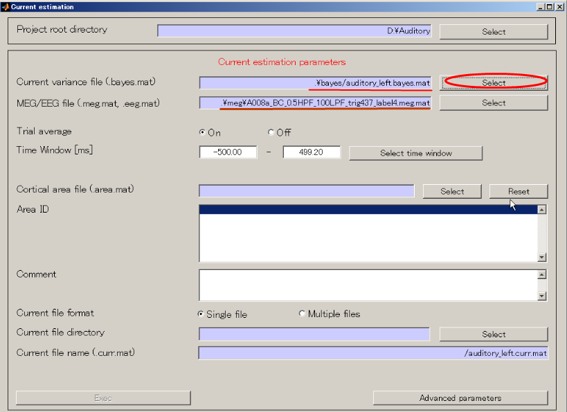
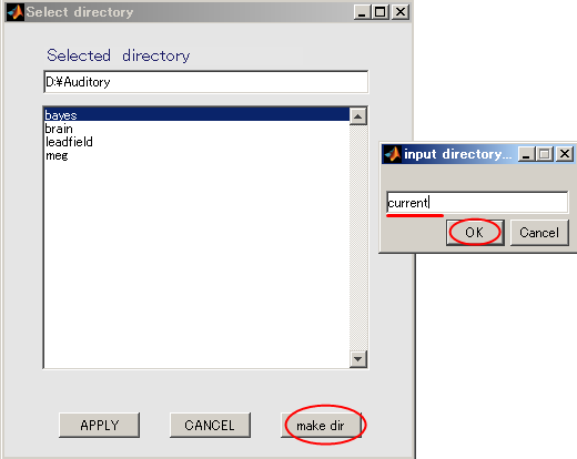
3. Specify the output destination(D:\Auditory\current).
   • Press Select button.

   
   
   

   • When you press the "make dir" button the dialog to input the name of the directory appears. Input "current" and press the OK button.

   
   
   

   • Click "current" and press APPLY.

   
   
   

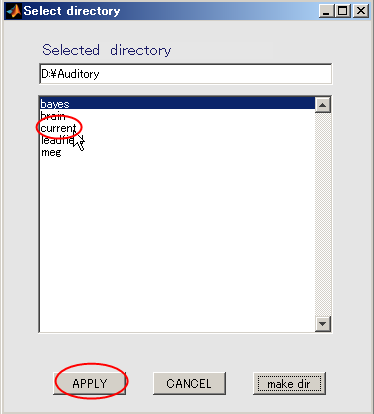
   • The output file name is updated.

   
   
   

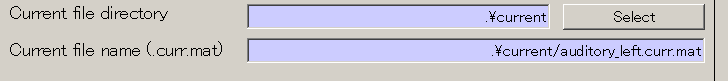
4. Press "Exec" button and the current calculation will be complete in 1 minute.

   
   
   <<MATLAB Command Window>>
   

    ----- New VBMEG -----
    Start current estimation
    Number of sessions: 1
    Time window: [1 1250]
    MEG data file for session 1: D:\Auditory\.\meg\A008a_BC_0.5HPF_100LPF_trig437_label4.meg.mat
    Number of sensors           : 400
    Number of trials            : 1
    --- Lead field matrix of focal window 
    Number of basis files (= Number of sessions): 1
    Area ID: Cortex
    Number of vertices: 20004
    --- Reduce cortex
    Number of reduced vertices: 4004
    --- Spatial smoothing filter calculation
    R = 6.00e-003, Rmax= 1.20e-002
    Number of vertices = 4004
    Number of vertices in expanded area = 20002
    Basis file for session 1: D:\Auditory\.\leadfield\A008a_BC_0.5HPF_100LPF_trig437_label4.basis.mat
     --- Save estimated current: D:\Auditory\.\current/auditory_left.curr.mat

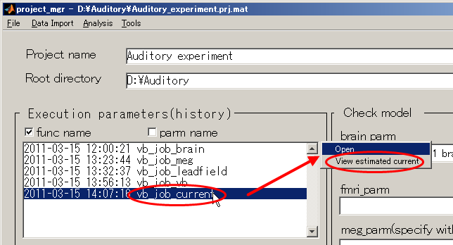
Viewing estimated current _

1. Return to the project_mgr GUI, click "vb_job_current" and then select

   "View estimated current" from the pop-up menu that appears on the upper right.
   
   
   

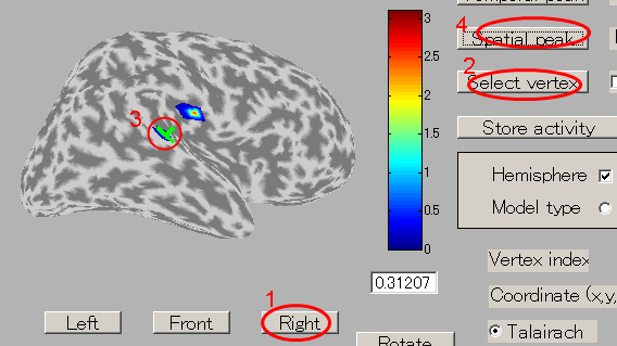
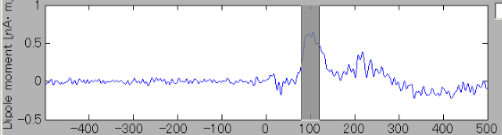
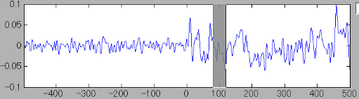
2. The GUI to show the estimated current will be displayed. In the spatial pattern display panel on the upper left of the screen, the average current intensity distribution for the selected time of interest (TOI) will be displayed on the inflated brain model. In the current time series display panel at the bottom of the screen, the current intensity time series averaged over the vertex included in the selected region of interest (ROI) will be displayed. The default size of the radius of the ROI is 4 mm.
   

   
   
   

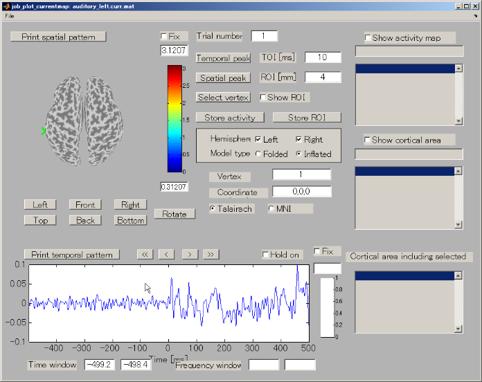
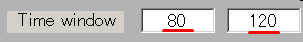
3. The TOI can be set by in the "Time window" field. Here, the TOI is set to 80-120 msec which is the latent time of the auditory evoked field (AEF) appearing in the both hemispheres.

   
   
   The current intensity spatial distribution is updated on the spatial distribution panel along with the setting of the TOI. The TOI appears gray on the time series display panel as shown below:
   
   
   

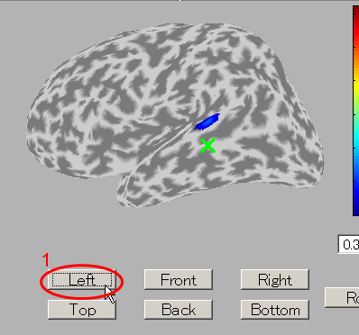
4. Press the "Left" button and you can see the cortical model from the left side. Brain activities are shown around the auditory region.
   

   
   
   

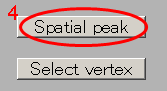
5. To select the center of ROI, press "Select vertex" button and then click one point on the cortical model. Here, the brain activity source around the auditory region of the left brain is selected.
   

   
   
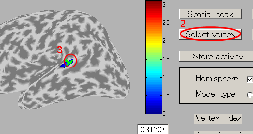
   The selected vertex index will be shown in "Vertex index" field.
   
   
   The ROI center can also be changed by directly inputing the vertex number to the "vertex index" field.
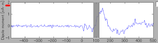
   The ROI center is indicated with green x-mark on the cortical model. Current time series of the selected ROI is displayed on the current time series display panel. The y-axis scale varies according to current time series.
   
   
   

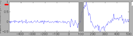
6. In order to find the vertex with the highest current intensity, press the "Spatial peak" button. The vertex with the largest time averaged current intensity will be displayed within the ROI and the center of the ROI will be set to this vertex.
   

   
   
   Simultaneously, the vertex number in the "Vertex index" field will be updated.
   
   
   The updated ROI current time series will be displayed on the current time series display panel.
   
   
   

7. The estimated current around the auditory region of the right brain can be shown through the same procedure.